In the past 9 blogs, I’ve shown you all sorts of Azure SQL database solutions and gave them a little run for their money. I’ve tested a lot and written about them. This blog will be about the summation of the data and my views on the combined graphs. At the end I’ll wrap it up with my way of working when a new project starts.
But before I kick off, a little Christmas present. What I didn’t do, until now, is give you access to more raw data. Now is the moment to give you more raw number to play around with for yourself and do your own analysis. Fun as it might be, I’d highly encourage you to use my sheets as a jumping point and adapt them for your own workloads. You can find the two Excel files via the link for the scripts.
Click here for information about the set-up
Click here for the scripts I’ve used
Let’s summarise the findings.
The results are all based on a small number of query’s. This means that the results are comparable between the different offerings, but most likely not to your workload. This may sound like an open door, but I want to protect you against inaccurate expectations. Any interpretation of results is coloured by the person interpreting the data. Yes, I do have opinions and as neutral as I try to be in my blogs, I will have coloured them with my working experience.
Technically speaking, there are a few main options. You can go DTU, CPU or Managed Instance. On a really high level, you’re choosing a magic mix between CPU, Memory and IO, a fixed number of CPU’s or a hosted SQL Server instance without the Windows Server. If you want more details, either check out my blogs on the different subjects or dive into the Microsoft Learn documentation. Remember that you switch between a large number of tiers, except two. If you want to change from Hyperscale or from Managed Instance, you’ll have to find a way to move the data out. You can’t change these tiers to another one.
Before you start out with all the goodies you can get, make sure you’re familiar with all the limitations. The good people of Microsoft have created pages where you can find all the specs and limitations, check these links out.
Related links:
Insert performance
As with all the blogs, let’s see how all the insert performance measurements compare with each other. I inserted one million records on 50 concurrent threads to see how quick the database could handle the traffic and the underlying index modifications.
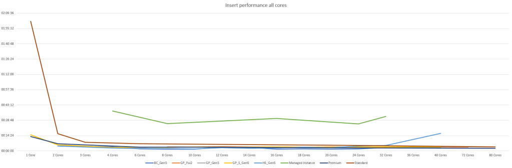
Don’t we all love the graphs where one outlier makes sure all the details are gone. It’s clear that 1 core on the serverless tier didn’t stand a chance. And yes, I’ve omitted the Basic DB because it would skew the results structurally. So, let’s drop the 1 core results to get some more detail.
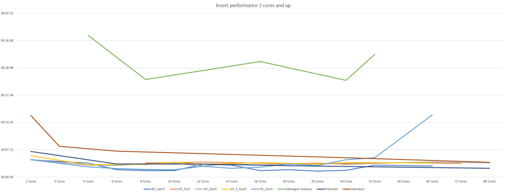
Now this offers a bit more information. It’s very clear that the managed instance tier is slower across the board. The other ones are quite close and though there are variations to be seen the extra hardware cost might not be justified to the performance gains.
The weird spike on the right is the Hyperscale 40 cores that for some reason didn’t want to ingest the data quickly any more. The spike from standard edition on the left was to be expected. You can’t expect a lot from a relatively cheap solution.
On average, inserting the data took 5 minutes and 33 seconds measured over 79 runs. If I’m adding the single core databases, the average goes up to 7 minutes and 11 seconds measured over 82 runs.
Just running all these scripts took 9 hours and 48 minutes.
Select performance
Let’s see what happens when I let my horrible query run. It’s been designed to sometimes use the indexes but most of the times there are only partly covering indexes leading to key lookups to complete the data. In some cases there are no indexes that trigger full index scans. Fun times for the engine.
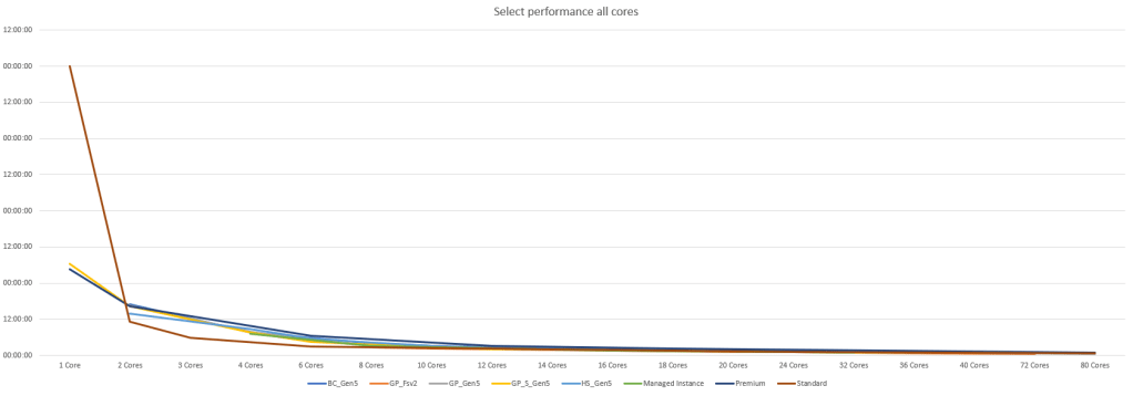
Just as with the insert, the outliers make short work of any details from four cores and up. The trend is already visible though, it all converges nicely at the higher end but let’s see if we can get some more details. I’ve dropped of the 1 and 2 core options and this comes up.
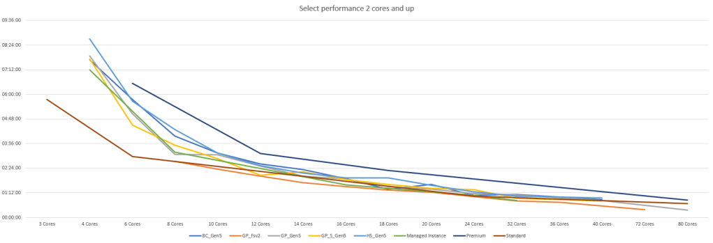
As seen in the detailed blogs, more hardware adds more performance but getting all the tiers and SKU’s together shows to me that it doesn’t really matter all that much which one you choose. The behaviour is quite the same across the board. As my query needs quite some compute power it’s no real surprise the compute optimised SKU finishes quickest. In this case, more hardware provides more performance when your database has area for improvement when it comes to indexing. Better indexing will surely help to get rid of key lookups for instance.
I’d strongly advise you to get a query of your own and test it out against a number of tiers and SKU’s to get a similar view as mine. Check the differences and define a KPI when the performance is good enough. If I’d want to run the query under one hour, I’d need at least 32 cores. But if one and a half hour is good enough, 16 cores will suffice. This will make a huge difference in my monthly Azure spend. As mentioned above, I’ve uploaded the Excel file with all the graphs to my github repository for you to play around with and modify to your own needs.
With all 82 measurements a total of 430 hours and 36 minutes was spent selecting the data, averaging at 5 hours and 15 minutes. Without the 1 and 2 core options, 73 databases are measured averaging at 2 hours and 31 minutes. Yes, the extra cores make a huge difference! The grand total drops to 184 hours and 6 minutes. The low SKU’s have cost me about 250 hours.
Update and Delete performance
As updates and deletes showed very similar behaviour, I’ve put them together in one graph.
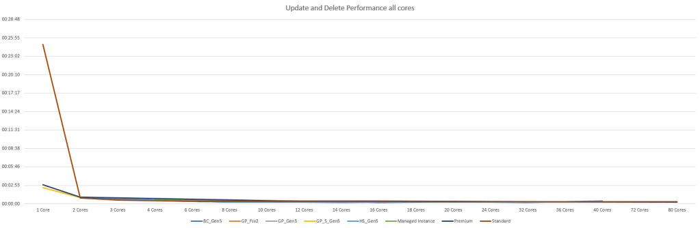
Well, this doesn’t say much other than don’t use standard on the 1 core SKU. Let’s drop it and see what happens.

There we go. No mush of lines but clear differences. The times on the left are in seconds, so the updates are quite quick all over the board. Yes there are differences but none of these are the decider for me.
With all the cores selected, the updates/deletes average at 45 seconds, racking up a total of a little over an hour. With the single core dropped, the average drops to 24 seconds and a total of 31 minutes. Again, the single core option has a huge impact on the average.
Pricing
Now the next thing we all want to know, how do all the prices compare to each other. Because at the end of the month, there will be a bill and you don’t want too many surprises. Your Azure SQL DB bill will be composed from a number of items. Not only the Tier and SKU you’ve chosen, but also the data size, backup options and your availability options. Because all these things offer too much variables to include in a chart I’ve omitted them and went for the tier/SKU pricing only with 32 GB of data.
The resulting graph:

The leader of the pack is the serverless option but you’ll surely remember that this one should only be used at 25% of the time. If you’re using the database more than that, go for the provisioned one. There was a discussion on Twitter lately about the moment the connection goes to sleep. You need to either close down the Object Explorer in SQL Server Management Studio (18 or 19) or fold in the databases folder in the object explorer. Of course a running query or transaction keeps the connection open as well.
The next most expensive option is the Premium option. But this again is calculated with full use whereas the DTU model is calculated on usage. If there are no running query’s you won’t spend as much money as this graph suggests. The Managed Instance and Business Critical are almost identical in terms of pricing but very different in performance and options.
Hyperscale and General Purpose are comparable on prices but there are major other differences. At the lower end of the prices we find standard and general purpose compute optimised.
Just for fun, on average an Azure database as shown here will set you back 3.331 euro’s. And that may be a very good figure to keep in the back of your mind. If you’re moving to Azure, aim for a range between 2500 and 3500 euro’s for just the database. Not storage, backups etc. Use it like the max degree of parallelism, start at 30 (OLTP) or 50 (data warehousing) and go from there.
What’s next?
So, with all this information, how to proceed. Here’s my way of working. First, I’m trying to understand the load that will be coming to Azure. Is it more IO or Compute intensive. Secondly I want to know the budget. Not an exact figure but a range. Then I try and explain how the costs are calculated, where the variables are and usually the range changes a bit. The next part is a proof of concept. Make sure it’s small and start out small with the resources as well. Scaling up is easier that scaling down and suddenly lose performance. Keep a good eye on the query store to see how things are evolving but run your own diagnostics as well. If you have a small dataset, scale the database down when you’re not testing. During my test phases, I’ve scaled the database back down to basic whenever I was processing results or working. Now you’ll probably be working with more than 2 GB of data so this one won’t be feasible, but the lowest SKU in the tier can be a cost effective alternative. We’ve even included this in a production environment where the ETL loads need a lot of oomph but the reporting can make do with much less. So we scale up when needed and down when possible. Remember that caches will be flushed when scaling so there is a disadvantage doing this as well.
Finally
This is the end of an 11-part blog series on 9 different tiers. The numbering went off with the first one and never recovered. It was a very enjoyable process to dig a bit deeper into all the offerings and gain more knowledge on them. It is so much fun to present sessions on this topic and listen to your experiences and what you’ve run into in your work. I really hope to continue presenting this session next year and let it evolve further.

One thought on “Azure SQL Databases part 10 of 9, round up”