I was teaching a class and during an interesting discussing an attendee told me that views with a filter took a long time to produce results, even if the result set itself was quite small. I wanted to test this out for myself to see what was happening. I’ll take you along this short journey in this blog. The outcomes have been validated against a SQL 2017, SQL 2019 and SQL 2022 instance.
Setup
First, let’s create the testing table.
SET NOCOUNT ON;
SET DATEFIRST 1 -- ( Monday )

CREATE SCHEMA DIM;
GO

CREATE TABLE DIM.DATE
(
	ID int identity(1,1),
	YEAR int,
	QUARTER int,
	MONTH int,
	DAYOFYEAR int,
	MONTHNAME VARCHAR(20),
	DAYNAME VARCHAR(20),
	WEEKDAY INT
);
GO

DECLARE @DATE datetime
SET @DATE = '2000-01-01'

WHILE @DATE <= SYSDATETIME()
	BEGIN
	 INSERT INTO DIM.DATE ([YEAR], [QUARTER], [MONTH], [DAYOFYEAR],[MONTHNAME],[DAYNAME],[WEEKDAY])
	 VALUES (YEAR(@DATE), DATEPART(QUARTER,@DATE), MONTH(@DATE), DAY(@DATE), DATENAME(MONTH,@DATE), DATENAME(WEEKDAY,@DATE), DATEPART(WEEKDAY,@DATE))

	 SET @DATE = DATEADD(DAY,1,@DATE)
	END
;
GO
CREATE OR ALTER VIEW vw_demo
AS

SELECT ID,
       [YEAR],
	   [QUARTER],
	   [MONTH],
       [DAYOFYEAR],
	   [MONTHNAME],
	   [DAYNAME],
	   [WEEKDAY]
FROM   DIM.DATE
WHERE [YEAR] > 2004
;
GO
This query will create a schema (not specifically needed for the demo, but as I’m mostly working in data warehousing, a schema for dimension tables is something I quite like.) Next I’m creating a simple table with an ID, a year column and a day of the year. Then a quick and dirty while loop to fill the table with some data. Let’s start without an index.
As the last step, I’ve created a view where I’m only filtering on dates that after the 2004.
First test, all the data
SET STATISTICS TIME, IO ON
DBCC FREEPROCCACHE

select  * from DIM.DATE

DBCC FREEPROCCACHE

SELECT * FROM vw_demo
If I run this query, I’m expecting the optimizer to only get the dates after 2007. For the output, it does. But let’s take a look at the runtime statistics:
 SQL Server Execution Times:
   CPU time = 0 ms,  elapsed time = 964 ms.

 SQL Server Execution Times:
   CPU time = 16 ms,  elapsed time = 929 ms.
Second test, add a filtering predicate
Not much of a difference there. One is filtering, the other one isn’t. So let’s add a second filter.
DBCC FREEPROCCACHE

select  * from DIM.DATE
WHERE YEAR > 2010

DBCC FREEPROCCACHE

SELECT * FROM vw_demo
WHERE YEAR > 2010
 SQL Server Execution Times:
   CPU time = 0 ms,  elapsed time = 567 ms.

 SQL Server Execution Times:
   CPU time = 0 ms,  elapsed time = 752 ms.
There is something of a difference here. It’s not much, but it’s not a large table. But almost 200 milliseconds difference is at least something. The execution plans are identical, just the scan of a heap table. The only difference can be found in the predicate:
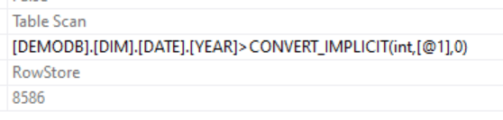
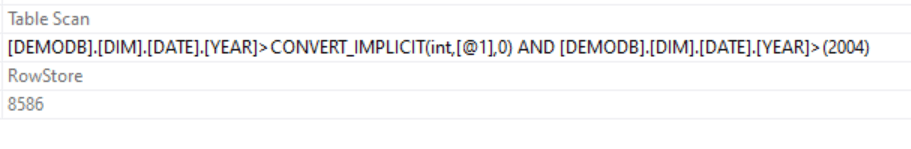
Where I’d half expected SQL Server to be smart enough and cancel the second predicate (as it’s useless compared to the first one) it didn’t. It just added a little extra work to the filter.
Now it may have something to do with the convert_implicit function that suddenly appears. I created the YEAR column as an integer and I’m providing the filter predicate as an integer. And still there’s an implicit convert.
Third test, remove the implicit conversion
So I tried this:
DBCC FREEPROCCACHE

select  * from DIM.DATE
WHERE [YEAR] > CAST(2010 AS INT)

DBCC FREEPROCCACHE

SELECT * FROM vw_demo
WHERE [YEAR] > CAST(2010 AS INT)
And look!

So, some extra syntax and I’ve lost my implicit convert from smallint to int. But does it help speeding things up?
 SQL Server Execution Times:
   CPU time = 0 ms,  elapsed time = 586 ms.

SQL Server Execution Times:
   CPU time = 0 ms,  elapsed time = 741 ms.
In this case, it didn’t help with any significance. I’ve ran the query a number of times and there are always small variations between executions.
Fourth test, adding a clustered index
Now, what would happen if this table had one index on the year column.
CREATE CLUSTERED INDEX CIX_YEAR ON DIM.DATE ([YEAR])
Let’s run the last query’s again and see what happens.
 SQL Server Execution Times:
   CPU time = 16 ms,  elapsed time = 509 ms.

 SQL Server Execution Times:
   CPU time = 0 ms,  elapsed time = 720 ms.
If anything, this only worsened the problem. The graphical part of the execution plan just show to index seeks, nothing special there. The properties reveal a lot more though.
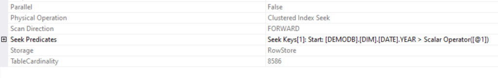
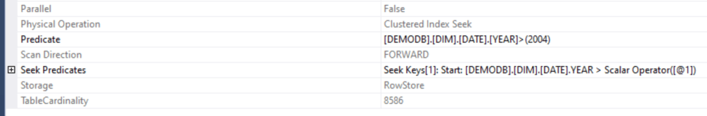
Both plans have the same seek predicates, but the filtered view also has it’s predicate in place. All the other properties are identical, it’s just this predicate that’s the extra part slightly slowing the query down.
Concluding
There is a difference in performance between getting data from a table or from a view where there’s already a filter in place. It depends on the table, indexes and query how much it matters. In my test case, the few milliseconds don’t matter. But if this table is being used in a procedure where this happens a gazillion times every night, even these milliseconds might matter.
Digging into rabbit holes like this one is one of the many reasons I love teaching classes. No matter how much I prepare, attendees can come up with the most wonderful questions and therefore enable me to learn even more. It’s never, ever one way.
Thanks for reading!

Interesting! I have always advocated against using views because of possible complexity. It’s just a stored query that adds complexity to the query that uses it. And manipulations of columns can make indexes (and statistics) unusable.
I can replicate your tests on a SQL2019 box with DB compatibility level 2019. Indeed the view query is slower.
I did some testing with several executions and then I find comparable average durations. What do you think of the below? I ran it on the heap table without statistics io,time on. I got an average duration of 71ms for the table and 68ms for the view. Apparently when running it more often (with re-use of the exec plan) it performs comparable. Note that the standard deviation of the durations are high. In my case it was about half of the average duration. And weirdly in my case: in almost all cases every 3rd or 4th execution of the query would be slower for both the table and the view.
drop table if exists dbo.results
GO
create table results(id int identity(1,1), mode nvarchar(10), startdate datetime, enddate datetime)
GO
DBCC FREEPROCCACHE
GO
declare @start datetime
declare @end datetime
set @start = getdate()
SELECT * FROM vw_demo
WHERE YEAR > 2010
set @end = getdate()
insert into results (mode,startdate,enddate) values(‘view’,@start,@end)
GO 100
DBCC FREEPROCCACHE
GO
declare @start datetime
declare @end datetime
set @start = getdate()
SELECT * FROM DIM.DATE
WHERE YEAR > 2010
set @end = getdate()
insert into results (mode,startdate,enddate) values(‘table’,@start,@end)
GO 100
select count(*) as #runs, mode,
avg(datediff(ms,startdate,enddate)) as avg_duration,
cast(stdev(datediff(ms,startdate,enddate)) as int) as stdev_duration
from results
group by mode
select *,datediff(ms,startdate,enddate) from results
LikeLike
The issue arises because your top-level queries qualify for simple parameterization (hence the @1 parameter markers).
The value inside the view isn’t parameterized, so you end up performing two separate comparisons in that case – once for the @1 value and once for the literal value 2004. Doing more work takes longer of course.
There are many ways to avoid simple parameterization where it is counterproductive. A common method is to add a redundant 1 = 1 predicate to the top-level query (not inside the view):
SELECT *
FROM vw_demo
WHERE YEAR > 2010
AND 1 = 1;
You could also add any meaningless query hint like OPTION (MAXRECURSION 100) or OPTION (KEEP PLAN). Since you’re clearing the plan cache between runs, OPTION (RECOMPILE) would also be harmless. As I said, any query hint will disable simple parameterization attempts.
Whichever method you choose, without parameterization the optimizer will collapse the two ‘YEAR’ filters on literal values into one equivalent test. Plans and performance for both approaches will then be the same, with both performing a performing a single test on ‘YEAR > 2010’.
LikeLiked by 1 person
Hi Paul, thanks for the reply!
I’ve tried it out and, the execution plans are identical now, both with the following seek predicate:
Seek Keys[1]: Start: [DEMODB].[DIM].[DATE].YEAR > Scalar Operator((2010))
Funny thing is, the regular query is still faster than the view with a filter in it.
LikeLike
May I invite you to reconsider your analysis? You are looking at elapsed time, but not taking into consideration the CPU time. If one query has to do more work than the other, it should show up in CPU time. The difference between CPU and elapsed is huge – what are the waits?
Also, I recommend looking at the query plans. Actual plans also give timing information nowadays, and are generally superior to SET STATISTICS TIME.
LikeLike
Hi Forrest, I think you’ve just set yourself up with a great introduction for your own blogpost :).
I did look at both query plans and, both were identical (as I wrote in the blog ;)). Getting waitstats on very short query’s is not impossible but it won’t give you much info. I tried it for you and, after filtering out all the benign ones (as per Paul Randall), the result set is empty.
LikeLike