Understanding Cross Workspace Data Transfer in Microsoft Fabric

When you open Fabric, the first thing you need to do is choose a so-called workspace. This serves as a container for all your Fabric items. You can have one or more workspaces and the design is entirely up to you. From one workspace to rule them all to one workspace for each set of items (Lakehouse, Warehouse, Semantic model and Report, Pipeline, Notebook etc). Until yesterday (the day this blogpost came online) it was impossible to use a pipeline to get data across different workspaces.

You could work around it with tricks like shortcuts, but it feels more natural (or maybe I’m just old ;)) to be able to read data from workspace 1 and write it into workspace 2.
So let’s see how this works and, where capacity is used!

Setup

I’ve created two workspaces. One is on a Trial F64 capacity, the other one a dedicated F2 capacity. As this blogpost has nothing to do with comparing performance (I’ve written more than enough about that ;)), I’m not going to copy a huge dataset. 90 million rows will suffice this case. I’m interested in how easy it works and moreover, where the capacity cost will be be.

Copy pipeline

I’m using a simple copy pipeline. I’ve created Lakehouses in both capacities.

The LH_CrossWorkspace is in my CrossWorkspace workspace, the LH_tpch is in my F64 Trial workspace. I can see both Lakehouses when I’m creating the dataflow in the F64 Trial capacity. Nice!

Chosen the source data, on to the destination. Again, I can see both Lakehouses and chose to load my data into a new table.

With this setting, let’s review it.

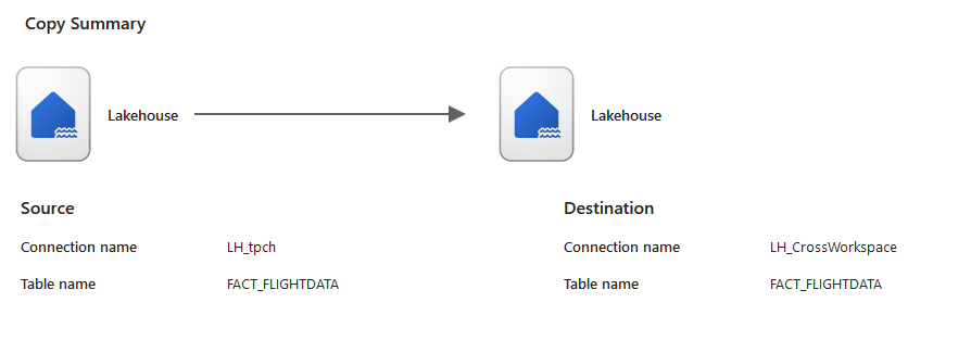
It would have been nice to see the names of the workspaces as well, but let’s suggest that to Microsoft. You will see it in the pipeline once it’s saved by the way, if the source or target is in a different workspace. It will be shown between brackets.

Running the pipeline

Well, it’s just save and run.

So it took about 5 and half minutes to transfer these rows. Which is less relevant this time as I’m more interested in the capacity usage as such. The pipeline is created on the F64 capacity and writing to the F2. But which capacity is used?

Capacity usage

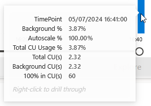
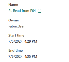
It took some time to become visible (about ten minutes) but then this showed up on the F64 Capacity.

It read data from the Lakehouse and that costs 2.14 CU’s. Cool, so let’s see what the other side thinks of this.

Nothing shows up on the F2 side. Now, as this pipeline is built at the F64 side, it reads at the F64 side and writes at the F2 side, it might not paint a complete picture. Why? Well usually when we transfer data between layers, it’s initiated from the layer where the data should go. So let’s see what happens when the F2 capacity is in the lead reading from the F64.

And now, on the F2 some usage appears.

Does anything show up on the F64?

Yes, weirdly.

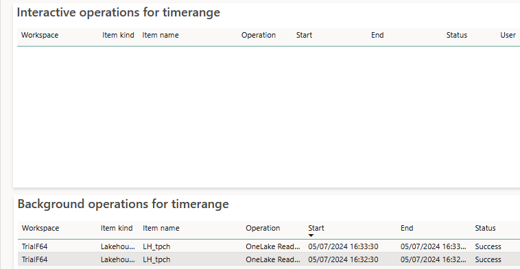
Let’s show the data as a table to see what was running.

It’s almost like there was smoothing taking place over a very low usage.

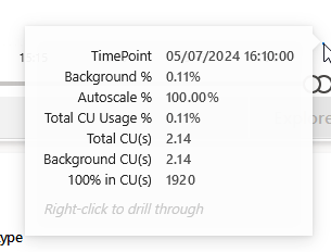
Digging into the latest time-point detail:

There were no interactive operations nor background operations for the selected point in time.

This hypothesis seems to be supported with these graphs.

Why? Well, the pipeline ran well before that point in time.

Notebooks as well?

Can you use notebooks from different workspaces as well?

You can switch the context of your notebook between Lakehouses, but a notebook is connected to a single Lakehouse and can’t read from one and write to another. If you’d like to have that functionality, vote for this idea.

Update july 6th 2024. I received feedback from multiple sources about options to use when you want to get data from one Lakehouse and write it into another.
The first option is to connect to the SQL Endpoint of Lakehouse and use that as a source. You can read all the data and process it in your data frame.
The second option is to use the abfss path to connect to the Lakehouse. This might need more work from the coding side of things, depending on what you’d like to achieve though. But there are alternatives to connecting your notebook to two Lakehouses in one go.

Concluding

Processing data between workspaces is easy now. You can select your preferred workspace as source and a different one as a target. The cost of the workload lies on the capacity where the pipeline is running. This includes the reads and the writes, irrespective of where the data is located. No matter the SKU and required capacity, you will be smoothed.

Notebooks are not yet able to do the same with ease, but there are valid alternatives you can use.

Thanks for reading!