Microsoft Fabric, comparing the F2 with the preview F64

If you’ve been having fun with Microsoft Fabric, chances are you’ve been playing around with the F64 capacity trial. This one is given to you by Microsoft for free but, since the GA data, the timer attached to it is counting down the days until you need to buy your own.

Most blogs I’ve read use this free trial capacity and it’s all fun and games there. The engine is quite powerful so most if not all tests will succeed. Which is cool but are you willing to pay the 8 to 10.000 dollars each month for this one? Granted, it comes with PowerBI licenses but still, a lot of money. If you want to read more on the licensing part, click here.
One small side-note on the cost; prices vary from the location where you deploy your resource. It’s the same for every resource but just keep it in mind when you deploy; if you’re not bound to a specific region, it can help to compare them to get the lowest price. I won’t post those comparisons here as prices are prone to change.

Testing methodology

To get a clear view on usage, I’ve been running processes sequentially. Things will change (a lot maybe) when your running them in parallel, like ingesting data, refreshing reports etc. Please remember that whilst reading on.
I’ve tested the F2 and F64 with the same source data, pipeline and notebook. The PowerBI part and Pipeline Gen2 will follow in a different blogpost.
The dataset is generated by the TPC-H toolset and imported ‘as is’. There is significant data loss but that is outside the scope of this blog.
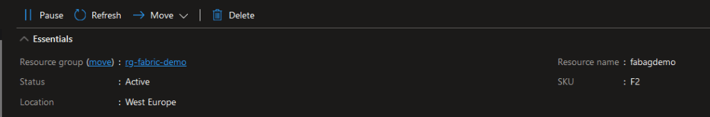
The F64 is the trial capacity from Microsoft that every admin can enable in their tenant. The F2 capacity is deployed in our own Azure tenant and paid for.
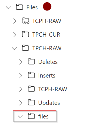
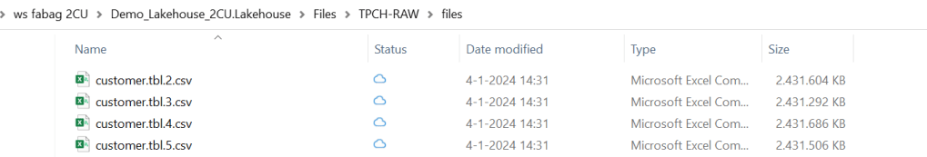
The original data is stored in an Azure Blob storage account without datalake setting enabled. The first ingestion step is a binary file copy where the CSV files are stored in the files section of the Lakehouse. The following steps use this files section to create tables in the Lakehouse.

Deploy Fabric capacities

There are two ways you can deploy Azure Fabric, either through the PowerBI portal experience where you enable the preview, or through the Azure Portal where you can choose the number of capacity units (CU). I wanted to compare both offerings to see if there are differences.

Now, when I wanted to create a workspace on my 2CU deployment, I got a message asking me if I’d like to enable the trial (and there was no option to decline). This was in august, I haven’t seen this question since. If you deployed Fabric at the time, right now you are running on the SKU you choose or set it to. Remember that you can scale the capacity up and down and pause when you don’t need it to run.

Let’s take a look at the settings within the Fabric portal. In the Admin portal, you can see the different capacity settings.

From this point of view, there’s a significant difference between the trial with 64 capacity units and our demo environment with 2 capacity units. The trial is 32 times more powerful. Or is it. That’s what this blog is trying to find out.

Dataset

To compare my workloads, I’ve used the same storage account (located in west europe, just like my F2 capacity) with the same CSV files. As mentioned in the methodology, these are the result of me running the TPC-H tool.

There are a few ways to compare the loads. At first I wanted to see how a notebook reads from an Azure storage account. And after reading some docs, I decided against that. Why? Well, authentication against the storage account needs a hardcoded access key (as Fabric can’t use a managed identity at the time of writing). And I think hardcoding keys is bad practice. So to get my data into my OneLake I could either copy it via my laptop (essentially killing the poor thing) or use a pipeline to just copy from the storage account to the Onelake.

Now, a keen reader would tell me that I’d still need a key, and they’d be absolutely right. The difference is that in this case, the key is obfuscated in the connection to the storage account. So it’s less bad. But you’re not here to read about me complaining on security.

Let’s try and find some differences between F2 and F64.

Pipeline

The pipeline itself is quite straightforward. Read the CSV in the storage account, write it in the Onelake. Job done. No extra settings, just a binary transfer.

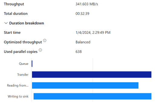
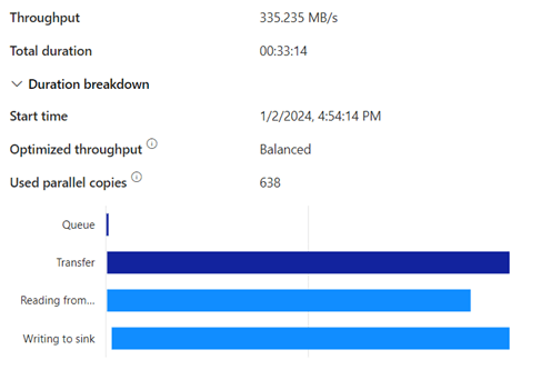
There’s a few seconds between them but that’s about it. Nothing to really worry about from this end. But what happens in my capacity? Because in both cases I’m using power to get the data in and this will consume power from my capacity.

Capacity app

If you want to dig into all the details of Fabric performance, you need the capacity app, a prebuilt PowerBI report that will give you a lot of information in one go. You can download the app here. After installing the app in a Fabric workspace, you need to connect it to a capacity you’re admin of. If there are more, they’ll all show up in the drop-down list of the app. I found that my F64 showed all the data immediately, the F2 needed about 12 hours to fully populate the app.

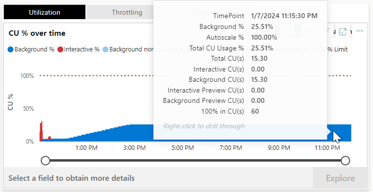
Let’s take a look at what this app tells me about the pipeline.

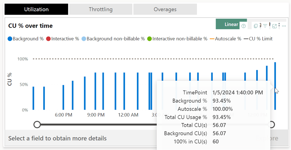
Ingesting the data might go at a similar rate, but it eats a much larger chunk out of your available F2 capacity units for the day. Or stated differently, processes following this ingestion might suffer from this process eating away a lot.
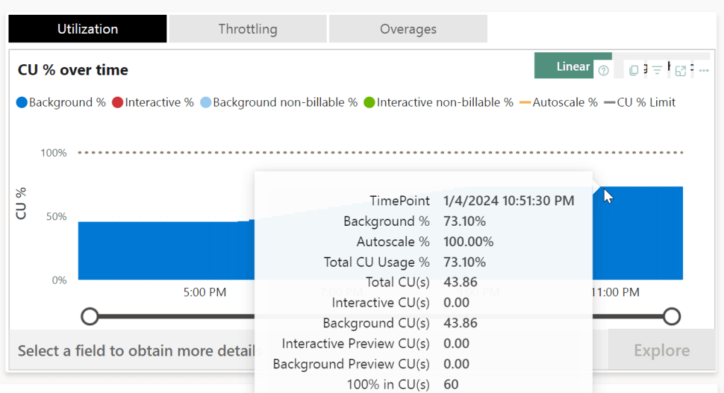
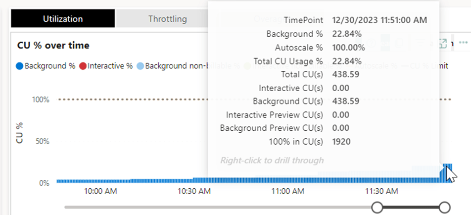
Ingesting the data costs 43 capacity units for that given moment in time. If you’ve got 60 in total (as you can see in the F2 screenshot on the last line; 100% in CU(s)), you’re using about 75% of your power available at that time. If you’ve got 1920 available (as you can see in the F64 screenshot), you’re using 2,2%.

These screenshots tell quite the story. Because now I can see the impact of my pipeline on the capacity. Time consumption is just one aspect. You need to keep track of these numbers to see what you actually need for your daily loads. If this would be all we’re doing here, F2 would just suffice, F64 would be over-provisioning. But usually, ingesting data is just one step of the daily work, so let’s see what happens when we mess about with the data a bit.

Transforming data from CSV to Parquet

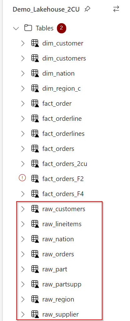
You can use a pipeline to transform the CSV to a parquet file, but that implies a data modification from the source. So my files section in my Lakehouse contains the raw CSV files, my raw table layer in the Lakehouse will contains the parquet files without any modification.

The file structure will differ, but the content will remain the same. Because I have to read from CSV and write to Parquet, I have to declare the schema; the column name and the data type. If you have a first line in the file as a header, you can infer the column names from there, else you need to declare them in the code.

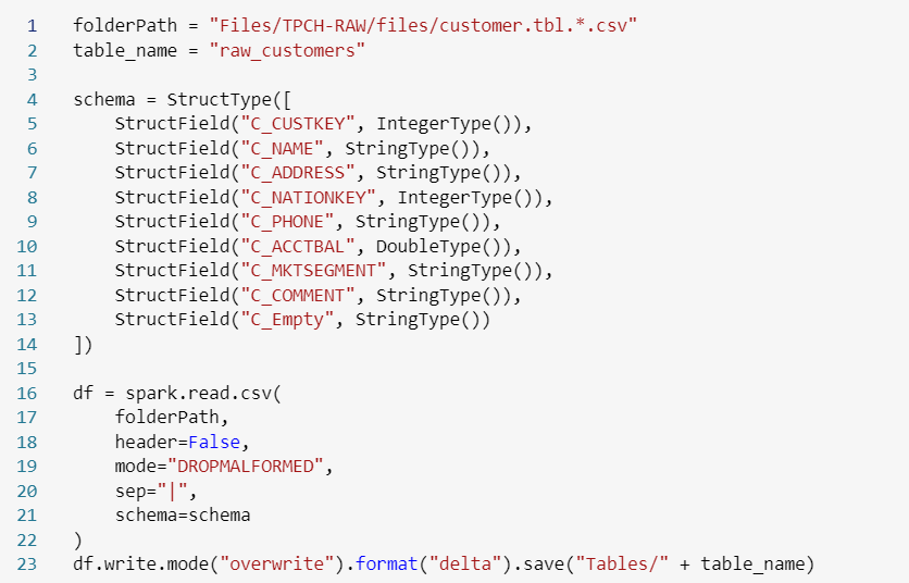
Code code reads the CSV file and writes it out in parquet files.

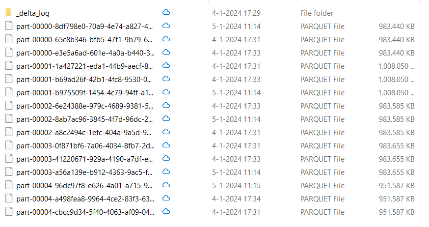
You can see quite the number of files with different timestamps. Well, it seems I’ve been loading the files three times, as the delta_log folder shows.

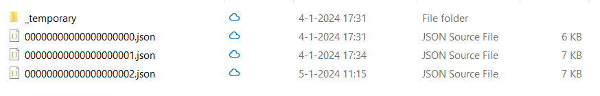
Now, this is just a small sidestep as you’re probably less interested in the amount of files and filesizes and more interested in the performance.

Right you are, let’s compare!

TableName	Number of rows	F2	F64	Factor
Customers	120.000.000	2 minutes 29 seconds	1 minute 13 seconds	2x
LineItems	4.294.965.612	2 hours, 4 minutes 55 seconds	7 minutes 46 seconds	17x

Again this comparison is just one part of the story, it’s just the runtime. When I’m loading at night when no-one is looking, it’s not the biggest deal if the run is 17 times slower. This will become an issue when report refreshes start failing because I’ve used all my capacity. so let’s look into that.

Capacity app

Looking at my work, this is the first thing that shows up.

I can see that my background usage is around 93 percent. But moreover, I can see that my F2 is limited to 60 CU’s and my trials have taken a little over 56 of them. Now this is, I think and at the time of writing, an essential metric. Because this metric informs me if I’m using the capacity to it’s limit or that I’ve got room to spare. Let’s compare it with the F64.

So my work here (with a little more retries making sure the number went up) shows that the F64 is nowhere near a breaking point. I’d even argue it’s waiting to break a sweat, working at 15%. The graph shows you that this F64 has 1920 CU’s ready to go, exactly 32 as many as the F2. Whereas I found that with increasing the SKU with Azure Sql databases there was less linearity to be found, scaling Fabric feels like a lineair process. At least the available capacity to run scripts. As we’ve seen in the above table, there’s no real comparison in duration between capacities and runtime.

Suppose you were running an F8 capacity, you’d have 4*60 = 240 CU(s). The above workload would fit in very nicely and run without major issues.

Modifying data

Let’s have some fun inside the Lakehouse; read data from a table and write it to another one.

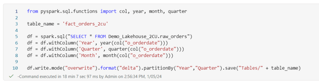
No, this isn’t a fact table, I know that. I just needed a name to stand out between all the other stuff.

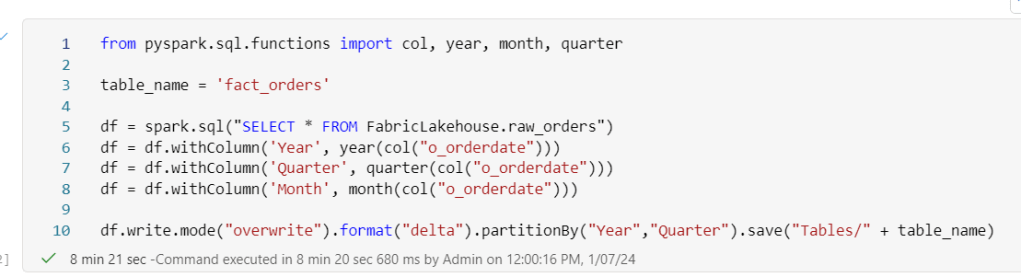
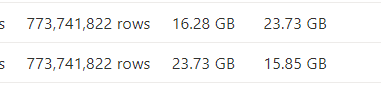
This process processes about 773 million rows.

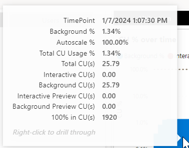
This process needs 25 CU(s) to finish.

So what happens when I start joining the two largest tables together.

Well, this is weird. I was expecting a huge CU(s) number on this process but it’s not all that much in the end. What does stand out is that the CU(s) usage is stretched out over the rest of the day; so my capacity lost 25% power during the rest of the day. This could be a sign of the smoothing/bursting process I’ll talk a little about in the next paragraph.

Let’s compare some numbers first

Script	Rows Processed	F2 Time	F64 Time	CU(s)	speed factor
fact_orders	773 million	18 minutes	8 minutes	26	2.25x
order_lines	4.2 billion	2 hours 16 minutes	2 minutes 39 seconds	15	45x

Smoothing and bursting

Now, let’s make things a little more complicated. Fabric has a technology called smoothing and bursting. To explain this effect, let’s use an analogy.
Suppose you’re driving along a road. It’s a nice day and there a section control over 20 kilometers where your average speed needs to be 100 km/h or less. When you’re over this, you’ll get fined. One way to achieve this is to drive along with 100 km/h and you’re good. Another way could be to drive around 120 km/h for the first half and 80 km/h for the second half, averaging at 100 over the entire distance.
The same holds true for the bursting part; you can go a bit faster for a period of time, just remember that later on, you will go slower to make sure the average matches. Most of the time, you probably won’t notice until you keep exceeding your CU. At some point Fabric will start to throttle you. From what I’ve heard processes will get queued or just slow down. In any case, end users will probably notice.

The other part of this story is the smoothing. Fabric will try to smooth the load of background processes out over a period of time. From what I understand at the point of writing it limits the risk of bursting and overusing the capacity. This is a balance I’d love to dig in deeper but will be something for a future blogpost.

So my poor F2 capacity got throttled. No wonder, I was trying to achieve this.

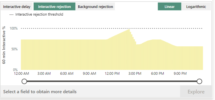
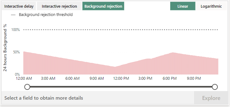
I was expecting more data from the interactive rejection and background rejection but probably because there was just one stupid notebook running with no interaction, the rejections stayed within bounds. Again something you need to test with your own workloads.

Combined workloads

If my daily run would mean I’d have to run both the pipeline and this notebook, I’d be using 43 and 56 = 99 CU(s). The F2 would struggle with that. The F4 might be a good fit as it will have 120 CU(s). This way you shouldn’t suffer too much from the smoothing/bursting part. But you need to take all the other processes into account and take a look at duration as well. If the processes are running at night this might be less of a problem, if processes need to do refreshes during the day; timing might get more important. And right now, the data is still stationary in the Lakehouse, not adding value. In the end, the purpose of the data is to add value to your organisation. Put differently, the data needs to be in a report for people to act upon.

Report

As mentioned in the introduction, I’ll get to the report and semantic model in a later blog. Why? Well, to create a report I need a semantic model. To create a report with a semantic model, I want to create my own semantic model and not use the default one from the Lakehouse. And for this you need to use PowerBI on your laptop. So far, no problem. But for some reason I can’t create a new semantic model, even though my account has a Premium per User license. Let’s file this one under lack of experience with PowerBI. Or maybe something else.

Final thoughts

Getting into the performance of Microsoft Fabric is an interesting journey. This blog is quite simple as it uses straightforward loads; nothing too fancy or difficult.

Microsoft Fabric uses smoothing and bursting to to prevent you from running out of steam on your workloads. This helps in finishing jobs but the rest of the day. you’ll be a little limited in your options. The numbers show that the bigger your capacity, the bigger the bursting and therefore the faster your loads finish.

My advice for you is to get a sample dataset that isn’t a small subset, preferably production size but anonymised. IF you make a mistake and publish your report to the world, it should make no sense to them whatsoever. Maybe I’m overly cautious, but with the never ending stream of data leaks in the news, make sure you’re not one of them.
If you can’t get a dataset from your company, use something like the TPC-H dataset to mimic your workloads and behaviour. Set up some schedules and get familiar with the capacity metrics app. Understand what the values are, what they’re telling you and what to adjust to make sure you get the most out of your capacity.

Something else to take into consideration is the data strategy of your organisation; if more and more people are expected to use PowerBI and the old P1 license gets into view, you can get the F64 license that contains the P1 PowerBI license. Maybe you’re all set within that one and all you have to do is add an alert when the capacity start reaching its limits.

Thanks for reading and I’d love to read your view on this!