I just can’t seem to stop doing this, checking the limits of Microsoft Fabric. In this instalment I’ll try and find some limits on the data warehouse experience and compare them with the Lakehouse experience. The data warehouse is a bit different compared to the Lakehouse, so I’ll be digging into that one first. Then I’m going to load data into the warehouse with a copy data pipeline followed by some big queries to test performance. The Fabric Capacity App will be used to check out the capacity necessary (or used for that matter).
As usual, I’m using the F2 capacity as it’s the one that should break the easiest. It’s also the cheapest one to run tests against and, as the capacity calculation isn’t dependent on the SKU (Stock Keeping Unit), you can easily translate to find out which capacity SKU will fit the workload. Remember that your workload will differ from the one shown in this blog. These tests are a comparison between the different offerings, something you could do for yourself. These blogs are a bit of a happy place as every option will get a good chance. In your work, your skills (and those of your co-workers) will be a major driver towards an option. Even if this offers the chance to learn something new!
But first, a short comparison and my view of use cases for the data warehouse.
Use cases
Before digging in, why would you start using a warehouse instead of a lakehouse? Is storage an argument? Not really as both experiences are loading data into the Onelake. In the lakehouse you’ll get some control over the files, the warehouse offers none; it’s all done for you.
When using a warehouse, you’re ‘limited’ to SQL. Most T-SQL commands we’ve come to know and love work inside the warehouse. In a lakehouse, there’s a more limited set available through SparkSql, but you get all the goodies from PySpark (Python), Spark, SparkR, and Scala.
There are some performance differences between the lakehouse and warehouse (which is sort of what this blog is about) but making the choice between these is also choosing a tool that fits your hand. If you’re well versed in T-Sql, there’s nothing holding you back from leveraging that knowledge and create an amazing warehouse inside Fabric. There’s no wrong and right, only different approaches to reaching your goal.
Now, I’m going to do some mad things to the capacity. The single intent is to exaggerate the errors and see when F2 will break. It’s not intended to knock the F2 capacity. But it’s the easiest to break and show you what happens when it breaks.
Test setup
To ingest data, I’ve chosen to read the CSV files from my Lakehouse. This saves me some hassle with ingestion from a different source.
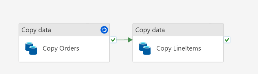
The first step is to use two copy flows and move data from the lakehouse to the warehouse.
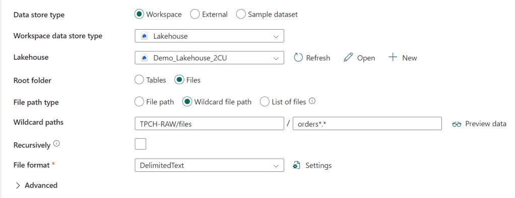
I’m using a wildcard to read the multiple orders files from the Lakehouse. The file format is delimited text:

Nothing special here, other than the pipe sign as the column delimiter.
The destination is my warehouse.

And the mapping:
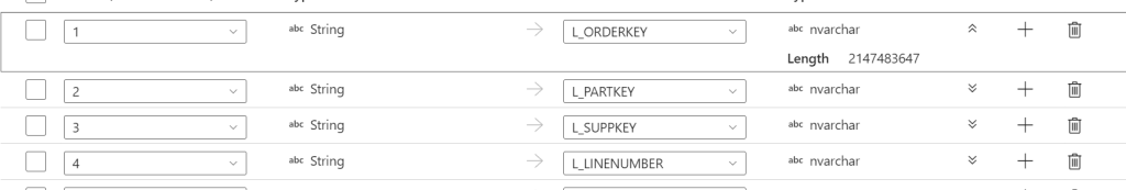
Now, the weird thing is that I can’t change my data types. They’re read as String and will be written as nvarchar without me having any control over length or even being able to cast them to another data type (something I can do in the notebooks). For anyone working with SQL, this is a bit nasty as incorrect data types can present all kinds of issues.
Finally, the settings for this copy flow:
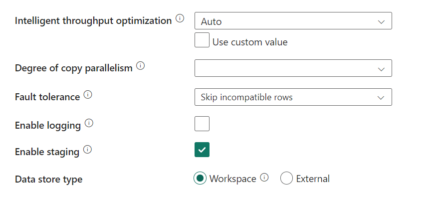
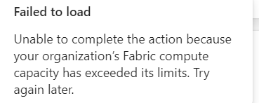
I’m skipping incompatible rows as I’ve seen that my CSV files aren’t all that healthy. One more reason to dislike flat files as a source but that’s beside the point of this blog. Something else is the checkmark at Enable staging. Because I’ve written in my Dataflow Gen2 blog that I don’t really like that part. But when I switch it off, this happens:
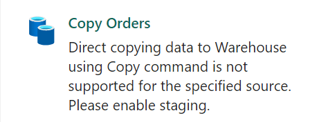
For some reason, staging is required. So, with staging enabled, let’s run the flows and see what happens when ingesting data into my warehouse.
Ingestion of orders
The orders table took some time but succeeded.

The funny thing is, from reading 90 GB of flat text data, the process wrote 103 GB of data. It created 368 files of about 200 MB in data. Instead of using compression (like the lakehouse does with the v-ordering, it looks like the ware house doesn’t do this.
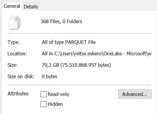
When I checked the folder later on, the actual stored data is less than the total amount of data written.
There’s a delta log as well:

From what I understand, these are regular parquet files represented as delta.
How much time does this take?
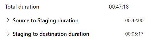
750 million rows in 47 minutes and 18 seconds. This translates to 258.888 records per second. That’s not bad at all! I’ve seen demos where inserting a few records takes seconds, but it seems the engine needs to warm up a bit because this isn’t bad at all! Although for comparison, the lake house notebook processed 120 million rows in 2 minutes and 28 seconds on the same F2 capacity, a performance of 810.810 records per second, a little over three times quicker.
Let’s zoom in a bit and see what happens within the staging part.

There’s some time to read from the source, a lot of time transferring data and then writing to sink (or destination as it’s now called).
The staging to destination was quite quick:
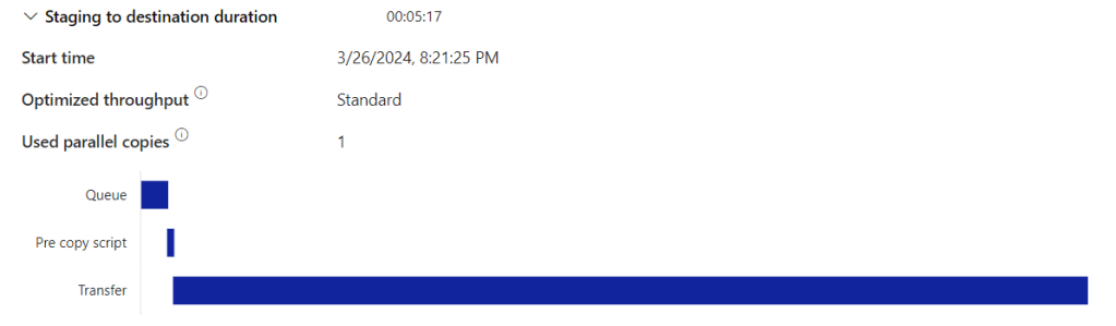
Let’s see how much performance it needed

Ingestion of Line Items
By and large the same story, bar one difference: parallelism. For some reason, the pipeline thought it was a smart move to use 6 threads to read 5 files. One of the threads hit a file that was already locked, and the entire process died because of it. So I had to set the parallelism to 5 manually. After some time, the load started to fail.
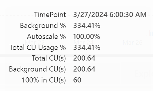
So let’s take a look at the capacity app. The total CU’s needed for this process are 200 where I’ve got 60 available.
Every now and then, the pipeline tries to let the outside world know it’s alive. But that’s about it.
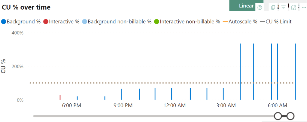
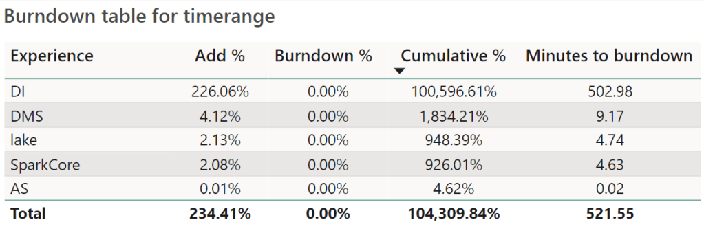
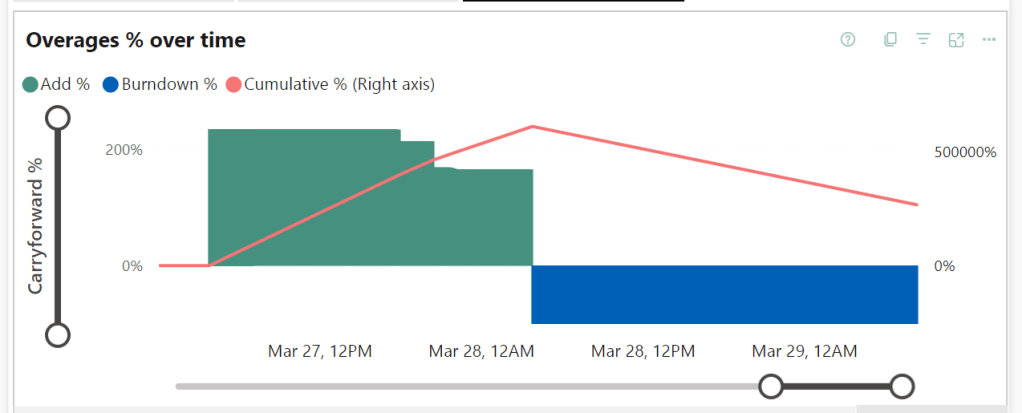
Looking at the overages graph, there’s a steep line towards long burndowns.
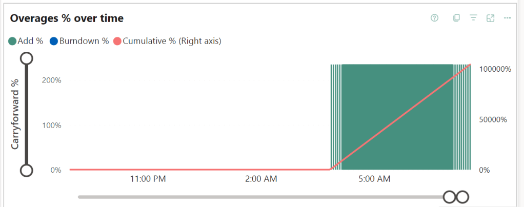
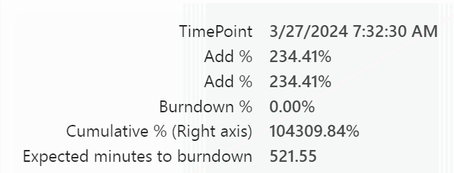
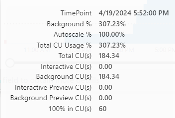
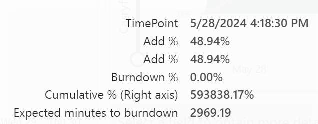
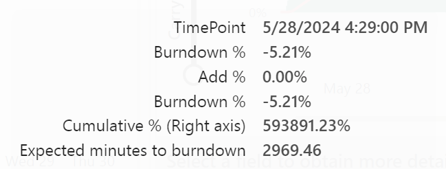
Let’s dig into the timepoint detail. There you can see that the overage just keeps adding at a 200% rate.
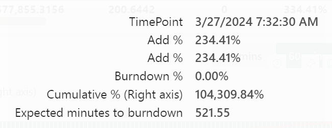
But there’s more.
Not only did I overuse the Data Integration, other elements are unhappy as well.
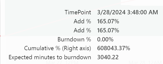
This screenshot shows the maximum point of my overage usage, leading to 50 hours of burn down after 24 hours of overage use. The net result is a Fabric capacity that is rendered useless for more than 3 days. This should be a signal that you’ve under provisioned your capacity and should increase the SKU. Nothing else. This really is just an example to show you how to test the limits. With an F8, the issue would have been way less or maybe even non-existent.
Now this process is taking quite some time. So I decided to pause the capacity and see what happens. Increasing the SKU can dramatically decrease burndown times and according to the docs, pausing the capacity will add the remaining cost to your Azure bill. So let’s see what happens.
Ok, overage use down to zero. Let’s give it some time (I need coffee ;)) and see what happens when I restart the capacity. But not after changing the flow a bit. Because if you repeat what you did, you’re most likely to get the same outcome.

Trying a different approach by loading each file in a separate copy item. Let’s see if this has a different impact on the capacity.
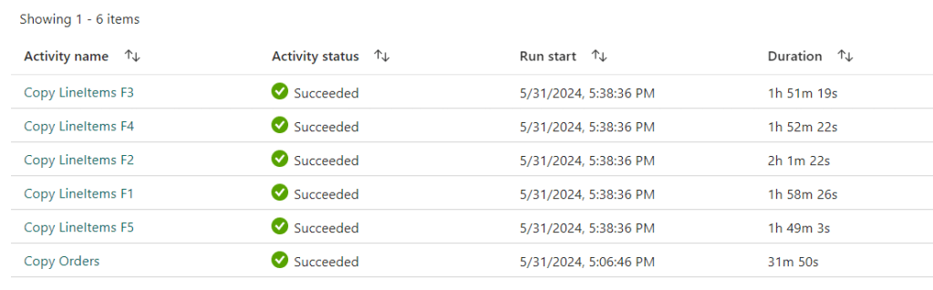
It probably won’t surprise you that the pipeline failed again. But less destructive this time, a few Copy data flows finished but most failed.
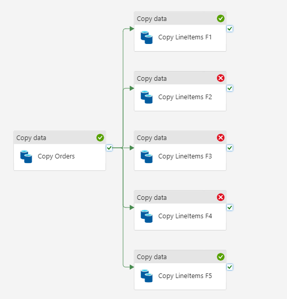
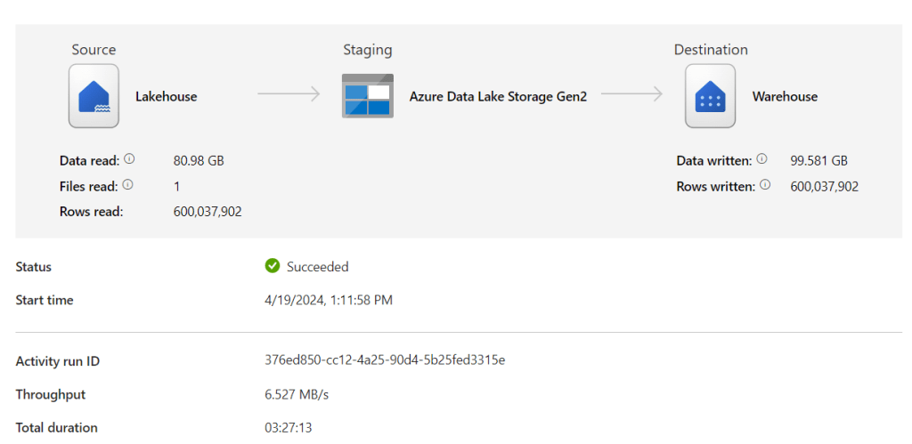
The succesfull part of this LineItems activity took 3 hours and 27 minutes to process 600 million rows.
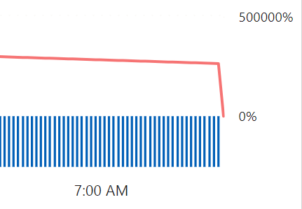
As expected, the bursting kicked in quite quickly and made short work of my capacity.

The drop at the end was caused by (again) pausing the capacity. This is a quick solve to make sure you can resume your work, though the left over capacity that should have burned down will be added to your monthly bill.
The copy activities running together needed about 185 CU’s where I have 60 available.
As I want the data in my Warehouse for the second part of this test, I upgraded the capacity from F2 to F8 and restarted the pipeline. Why the F8? As the feedback from Fabric is that I need thrice the capacity available with an F2, In theory an F6 would do the job. If it would exist. As it doesn’t, the closest one available is the F8. An alternative would be to keep redesigning the pipeline until it would fit the F2. But let’s be honest here, this volume just doesn’t fit in an F2. And, I’ve learned that the pipelines just consume more capacity working in parallel.
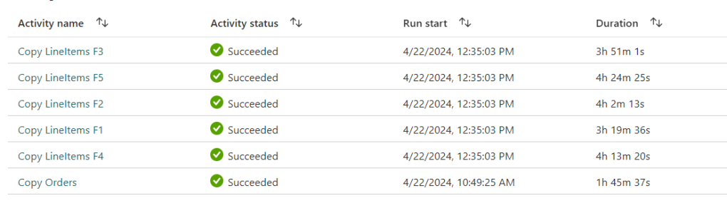
So yeah, using an F8 worked to get all the data across; 1 hour 45 minutes for the Orders and 4 hours 24 minutes in total to process all the LineItems coming to a grand total of 6 hours and 10 minutes to move the CSV Files into the Warehouse with a pipeline. As a side note, the F2 capacity finished transforming the files from CSV to Parquet in a Notebook after 2 hours and 5 minutes.
Now I can move to the second part, selecting data in the Warehouse and creating new tables. Of course, this is done on the F2 capacity to check what it can handle.
Running queries
So let’s start with some easy queries against the warehouse, doing some counts.
SELECT count_big(1)
FROM dbo.LineItems
-- 4.200.082.323 1 second 676 ms

SELECT count_big(1)
FROM dbo.Orders
-- 2.250.000.000 1 second 445 ms
Wait, the orders only have 750 million rows, right? Yes, but I wanted to get the time needed for ingesting both tables in one run, including the needed capacity. With multiple runs, the data just gets added to your table. Something to just be aware of, overwrite doesn’t happen automagically.
Let’s get the distinct data from the orders table, write it to a different schema and add some columns based on the OrderDate column.
SELECT DISTINCT
    O_ORDERKEY,
    O_CUSTKEY,
    O_ORDERSTATUS,
    O_TOTALPRICE,
    O_CLERK,
    O_SHIP_PRIORITY,
    O_COMMENT,
    YEAR(O_ORDERDATE) as O_OrderYear,
    DATEPART(QUARTER, O_ORDERDATE) AS O_OrderQuarter,
    MONTH(O_ORDERDATE) AS O_OrderMonth,
    DAY(O_ORDERDATE) AS O_OrderDay
INTO DIM.Orders
FROM dbo.Orders
I was half expecting this query to fail. But!
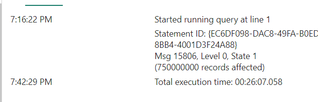
It actually processed the 750.000.000 rows in a little over 26 minutes. The notebook needed 17 minutes. But it got through it and that’s not bad at all!
Now the big one, joining the order lines (4 billion of them) to my orders.
SELECT *
INTO FACT.OrderLines
FROM DIM.Orders O
left outer join dbo.LineItems LI on O.O_ORDERKEY = LI.L_ORDERKEY
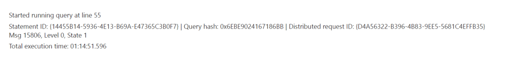
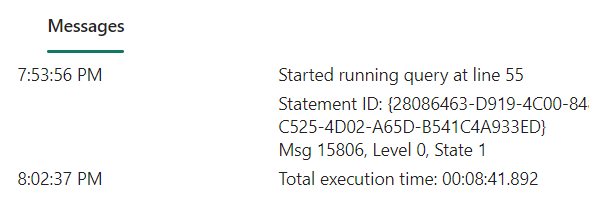
The funny thing is, the query finished ok it seems, but there’s no row count. When editing the query window in Fabric, this message shows up.

Are there rows in the table though.

12.600.246.969 rows. Even though I deleted the table in between. so let’s dig into the files themselves, because this is unexpected.
To do this, I’m using the Onelake File Explorer, a preview tool you can download to get browse through the files inside Onelake as if it were your Onedrive.

I can see many files, created between 15:24 and 17:31 with a filesize between 3 and 153 MB. This suggests that the runtime of the query itself is 2 hours and 7 minutes. Assuming the timestamps are directly related to the runtime.
After this little sidestep, let’s dig into the Metrics app and see what lies beneath.
Metrics app
Let’s see what the metrics app can tell.
The first time I ran this query it went a little over the capacity but not all that much. But, doing that for a little over an hour does build up some overage that, as I found out, kept on building. But as these results were a bit weird and inconclusive, I ran the query again (and again) as requested by the Fabric Team to see what’s happening.
The utilisation graph is filled some more, but it’s still missing a lot of data points.
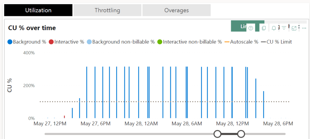
There is a clear pattern when it comes to the bursting, the query clearly goes well over 100% of the capacity but it seems to limit at some point.

Let’s zoom in a bit and check out what’s registered during the time the query was running and writing files (as seen in the Onelake Explorer).
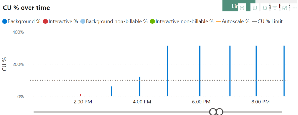
Now the lack of data points really starts to hurt. In the beginning, the query doesn’t need all that much capacity. Around 16:00, it start’s to go over the limit and at 17:00 it comes to the maximum it needs. The thing is, a little after 17h, the query itself finishes, but the utilisation keeps on running.
Important message!
Remember this, based on utilisation alone, you cannot identify long running processes. You need to know what was running at the time and start digging in deeper. You can do this by right-clicking on the time point and drill through.
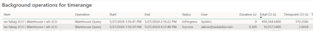
You might see something like this, after sorting the table. One operation in progress taking an immense amount of CU’s. Though with different timestamps and, when I checked on a different time, the result in the metrics app is identical. Which is weird. My gut feeling is that I’m doing so many weird things to the capacity that the capacity metrics app loses track as well.
Let’s say my query to join the lineitems to the orders table is three times as heavy compared to what the F2 has to offer. This means I’m running into my overage again.

My overage usage started at may 27th 15:33 and ended may 28th at 16:18. Consuming data from the future. Almost 25 hours of overage for a query that ran about 2 hours. How long did it take to burn all that usage down?

The burndown started May 28th at 16:29 and finished may 30th at 18:04. It took around 50 hours to get back to normal. In total my capacity was declining any request for 75 hours. Because I was hammering it with too much work. Or, too much work for the Warehouse experience to cope with.
What about F64
Well, just to give you some extra food for thought, I ran the pipeline against the F64 Trial.

Combined with the LineItems:
All the processes were running in parallel leading to a total time of 2 hours and 32 minutes to ingest all the data into the warehouse.
So let’s see what the data warehouse engine can do.
8 minutes to join the two tables?
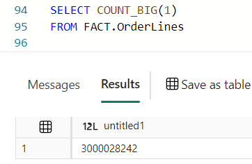
3.000.028.242 rows. So 1/4th of what the poor F2 had to do. But still, if this scales linear and add some time for overhead, about 4 times this is 36 minutes. Way quicker than the F2 with two hours or more. On the other hand, it’s ‘only’ 4 times faster with 32 times more power.
Compare them
Ok, let’s do a quick comparison between the F2 and F64 Warehouse and Lakehouse experiences
| Lakehouse CU | Warehouse CU | Lakehouse Time | Warehouse Time | |
| Ingest F2 | 43 | 364 | 00:32 | 04:10 (failed) |
| Ingest F64 | 43 | 364 | 00:33 | 02:32 |
| Transform F2 | 15 | 342 | 02:16 | 02:10 |
| Transform F64 | 15 | 342 | 00:14 | 00:36 |
For me, this shows that ingestion (done both in Lakehouse and Warehouse) is much more efficient into the Lakehouse. The warehouse just takes much longer, something that could be related to the amount of files.
For the transformation, I’m showing the amount of time 12 billion records would have taken for the F64. The amount for 3 billion was 8 minutes, close to 50% faster than the Lakehouse. But that comes at quite a price looking at the CU’s.
So, now what?
Very good question! First of all, you shouldn’t do this. Hammering your F2 with these amounts of data will just fail. It’s nothing you can hold against Fabric. It is however very important that you start testing your loads at an F2 capacity and see where the pain begins. Because maybe running the entire load on an F8 capacity saves you all the issues I’m seeing here. As you’ve seen with the pipeline ingestion, scaling up to F8 solved the ingestion issue. Yes, it’s 4 times more expensive than the F2, but it gets the job done. Now it’s your choice what’s more important. Or, you could use a Lakehouse to ingest your data and use that as your starting point to process data in your Warehouse.
The second, harder question is, should you use the data warehouse experience. That depends. First of all, it depends on the people in your organisation. If they are fluent in SQL and hardly speak PySpark, it’s obvious to work with the warehouse experience. You could invest in your people learning PySpark for the longer term.
Second, it depends on the complexity of your ETL/ELT processes. If it’s quite straightforward, the data warehouse can cope. When it gets more complex, I’d advise you to take a look at the Lakehouse to get the best value for money.
It also depends on your data architecture. If you’re running an Enterprise Data Warehouse, it’s usually fully SQL based. If you’re moving to Modern Data Warehouse, you’re moving towards Lakehouses combined with a Warehouse. When you’re going for the Data Fabric, you’ll have the added joy of real-time analytics as well. There are no wrong or rights here, nor are there hard boundaries.
At the beginning of this blog, I started out with comparing the warehouse and Lakehouse. Now that you’ve reached the end, it’s hard to do that comparison based on numbers as the warehouse has issues with the F2 that the lakehouse frankly doesn’t have. But it’s also unfair to state that the lakehouse is 4 times stronger than the warehouse. In my very specific case it is, but you can’t make a generalisation like that.
In the end, your choice of tooling and experience should be based on the knowledge and expertise in your organisation. Just make sure you base your choices on metrics, coming from your data and processes, not from some guy writing blogs 😉

Hi,
Great description.
I am wondering about the capacity storage.
In Warehouse, a backup (restore point) is made every 8 hours and their retention is 30 days, which gives 120 copies of data. If your data is 100GB, the total WH will be 1.2TB.
How does this compare to Lakehouse, where you have a vacuum for, say, 7 days but you make ingestion 3-4 times a day?
regards
Przemek
LikeLike