
Welcome to my blog series on Azure SQL DB performance. In this blog I’ll write about my findings with the Azure SQL DB General Purpose Provisioned tier. Quite a mouth full.
Click here for information about the set-up
Click here for the scripts I’ve used
Intro
In my previous blog, I wrote about the serverless tier, the one that can go to sleep if you’re not using it for more than one hour (minimum). That tier is cheaper as long as you’re not running it for more than 25% of the time. If you need more time, go provisioned.
Another difference between serverless and provisioned is that the provisioned one gets a set number of cores whereas the serverless one has a minimum and a maximum number of cores. So this time, the blog is about the provisioned tier where you choose a fixed number of CPU’s with a fixed monthly cost.
Limits
The provisioned tier starts at 2 cores as a minimum and goes up to 80.
The maximum storage starts at 1 TB and goes up to 4 TB. The number of TempDB files is undisclosed but the size is and starts at 64 GB At the top end it goes a little over 2 TB. The disk limitations are disclosed as well. Log rate starts at 9 Mbps and maxing out at 50. The same goes for the data; starting at 640 iops and maxing out at 12.800. One iop (or Input Output oPeration) is connected to the disk cluster size. As these are 4 kb, reading or writing one data page (8Kb) equals two iops. 640 Iops equals something of 2 MB per second. The top end goes to about 50 MB per second. Keep this in mind when you’re working out which tier you need, because disk performance can be essential.
When you compare these numbers with the serverless tier, you can see that at the bottom end, the limits here are double the limits of serverless.
Resources provided
I’ve deployed all the standard options and got the following results:
If you’re looking at these numbers, there are quite a few weird things happening.
SKU | Memory | CPU Cores | Max workers | Schedulers | Scheduler total count |
| GP_Gen5_2 | 7 | 2 | 32 | 2 | 11 |
| GP_Gen5_4 | 16 | 4 | 32 | 4 | 12 |
| GP_Gen5_6 | 25 | 6 | 32 | 6 | 14 |
| GP_Gen5_8 | 34 | 8 | 26 | 8 | 19 |
| GP_Gen5_10 | 43 | 10 | 32 | 10 | 18 |
| GP_Gen5_12 | 52 | 12 | 32 | 12 | 23 |
| GP_Gen5_14 | 61 | 14 | 64 | 14 | 22 |
| GP_Gen5_16 | 70 | 16 | 32 | 16 | 24 |
| GP_Gen5_18 | 79 | 18 | 64 | 18 | 26 |
| GP_Gen5_20 | 88 | 20 | 64 | 20 | 31 |
| GP_Gen5_24 | 108 | 24 | 64 | 24 | 32 |
| GP_Gen5_32 | 147 | 80 | 20 | 32 | 99 |
| GP_Gen5_40 | 172 | 128 | 32 | 40 | 149 |
| GP_Gen5_80 | 353 | 128 | 32 | 80 | 142 |
Memory and CPU start to increase at a steady rate at the bottom but go wild at the top end. The amount of schedulers, that in my opinion determines the amount of work the database can do, has a much more balanced growth and are in line with SKU description. Every scheduler is ‘bound’ to a cpu core. It should be that the amount of schedulers represents the amount of cores. Yes, there are hidden schedulers but these should be hidden from the used view as well.
The amount of workers on the other hand is a bit wonky. I have no idea what’s causing this behaviour and I’ve seen different results with identical deployments. When we look at query performance, there might be a relation between performance and amount of workers. The workers are the ones doing the work for the schedulers. But with less workers, the schedulers seem to be done.
One way of checking if the the workers and schedulers can change in your favour is by changing the SKU as far up as it can to see if you can get it to move to another node. Then change back down to your preferred SKU and check the results. It isn’t pretty but it might be quicker than submitting a call to Azure support.
Running query’s
We’re not using a database to sit around idle, we need to insert, read, delete and update data (in whatever order you fancy). When you look into the code post, you’ll find the scripts I’ve used to do just that. Insert a million rows, try and read a lot of stuff, delete 300.000 records and update 300.000. The reads, updates and deletes are randomised. Because of the large number, I think the results are usable and we can compare them between tiers and SKU’s.
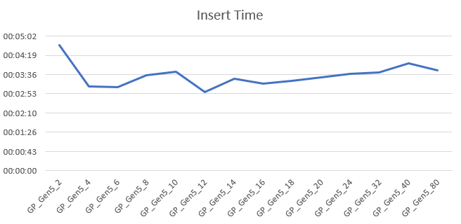
Insert 1 million records
I’ve insert the records on all SKU’s within this tier. With 2 cores, this took 4 minutes, from 4 cores and up it was done between 3 and 4 minutes. It’s funny that increasing cores doesn’t add any extra insert performance. What it does prove is that throwing more hardware at your solution doesn’t necessarily improve performance. When running these query’s, I noticed that the process goes off to a flying start and then slowly reduces speed the more changes have to be done to the index. The larger the index grows, the more time it takes to add data to the page or shuffle pages around to keep everything in order.
Wait types I’ve seen the most:
This isn’t a long list. Yes there were more, but with less than 1 percent of the total wait time I opted to skip them. The inserts are waiting on the logging for almost half of the time. Do not underestimate the impact of this wait. You can’t switch to simple recovery to mitigate this one. In three of the fourteen cases, I’ve had the VDI wait. The total wait time amounts to 35%. When you’re changing tiers, this will come up. When it occurs, it’s there to stay for some time. The other waits are expected, getting exclusive and share latches on the pages that need to be written. As usual, the extended events waits pop up as well to populate the portal graphs.

The read and write latency varied between 2 and 53 ms, averaging at 34ms read and 4.7ms write latency. It really varies and has hardly a relation with cores. Depending on your workload, this can be either something do dive deep into or to keep in the back of your mind.
Select data
After inserting data, it was time to select some. The script that I’ve used is intentionally horrible to make the worst of the performance. The 2 core DB took 16,5 hours to complete. Just like the inserts, you can see enormous increases at the low end but the more you increase, you get less extra performance. The 80 core SKU finished in just over 22 minutes. Like the previous graph, the more cores you add, the less extra performance is gained. But every core added does increase performance. Every time we double the amount of cores, the time needed to complete is halved. That’s quite impressive to be honest, because there hasn’t been any tuning and the runs are always fresh; no cached plans for example.

The wait types I’ve seen the most:
- SOS_SCHEDULER_YIELD
- CXPACKET
- CXSYNC_PORT
- VDI_CLIENT_OTHER
- LATCH_EX
- RESOURCE_GOVERNOR_IDLE
- XE_LIVE_TARGET_TVF
This time round the waits are on reaching the maximum time a query can spend on the processor (4ms). This was almost 33% of the time over all SKU’s. Next up parallelism. These waits became more prevalent in the higher SKU’s with more cores. Note that you really need to keep your parallelism in check, or allow for these waits. Even after getting through inserting all the data, the database was still busy with everything needed to change the database SKU. Getting exclusive access to data pages to about six percent of the time, the resource governor (the way Azure is limiting the resources on the databases took about four percent of the wait time. These were higher in the low end and less in the high end. The xe_live_target_tvf wait amounts to about 1 percent of the wait time. It’s good to know it does take some time though it shouldn’t interfere much with your running query’s. Yes there were other waits but with under one percent of the total I’m discarding them for now.

The read latency was anywhere between 18 en 57 ms, write between 4 and 69 ms. The latency averages a6 35 ms for read and 23 ms for write operations. The only reason I can think of why write latency increases at the high end is that more information per second can’t be handled by the disk when writing to disk for sorts. When looking at the graphs there seems to be a sweet spot at 12 and 18 cores. But as with all these blogs, test for your own workload to find the sweetspot(s).
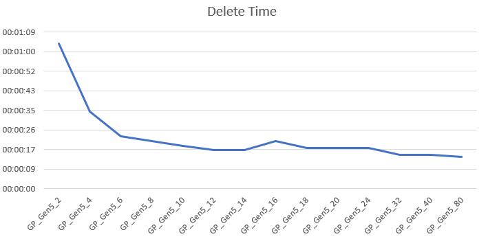
Delete data
After selecting data I decided I had enough of the large amount and had to trim some of. So I deleted 300.000 records. This process is quick all over the board, ranging from a little under 1 minute for the 2 core SKU minutes to 14 seconds at best. The gains from 6 cores and up were very little as you can see in the graph. Just like the DTU tiers, at some point adding more cores doesn’t really help anymore.
The wait types:
- WRITELOG
- XE_LIVE_TARGET_TVF
- PWAIT_EXTENSIBILITY_CLEANUP_TASK
- PVS_PREALLOCATE
- RESOURCE_GOVERNOR_IDLE
- PAGELATCH_EX
- PAGEIOLATCH_EX _
Well there are many surprises here, for me at least. The serverless SKU was mostly waiting on exclusive access to the datapages, here the access only takes about 4% of the wait time. About 50% of the time is spent waiting on the log file. Of course there are waits on the eXtended Events for the portal racking up 17 percent of the wait time. The PWAIT wait type has to do with SQL Server Machine Learning services. PVS Preallocate is a background task that is sleeping between preallocating space for the accelerated database recovery service. It sounds benign enough to ignore. For about 3 percent of the time, the resource governor was slowing down the work to make sure everything stayed within the boundaries of the chosen SKU.

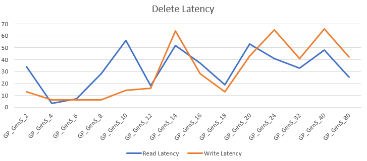
The read latency varied between 3 and 56ms, the write latency 6 and 56ms. Just like with the serverless tier, the latency went all over the place. I’m hesitant to add any conclusions to these numbers because of the short duration of the query’s. The latency averages at 32 ms for read and 30 ms for writes, both higher compared to serverless.
Update data
The last job I let rip on the database was an update task. I ran a script to update 300.000 records. The 2 core took 1 minute and 6 seconds, from the 6 cores and up went around 20 seconds where 40 and 80 cores showed serious improvement with 14 seconds runtime. The behavior is quite the same as with deletes.

Let’s take a final look at the waits
The main wait is again exclusive access to a datapage to modify it. This wait took almost 85% of the time. Second is waiting on the eXtended Events for 7 percent of the time. Third is waiting on the launchpad service that has to do with SQL Server machine learning services, but only 4 percent of the time. The last one is the resource governor holding us up for a little over one percent of the time.
The latency is comparable with the update graph. Read between 3 and 56 ms, write between 6 and 66 ms, averages for read 32 ms and write 30 ms. Again both a bit slower than serverless.
Pricing
The pricing shows a quite stable line up to 24 cores. When you’re choosing 32, 40 or 80 cores, the price graph becomes somewhat steeper. But all in all it should be quite predictable where you’re ending up. But your companies credit card might start smouldering a bit.

More performance will cost more and you’ll have to decide if this tier and it’s SKU is worth the cost. To keep this under control I’d advise you to use the cost center and it’s alerts. Not only the actual costs, you can create cost alerts on predicted costs as well to prevent surprises. We’ve all been there.
Finally
For our data warehousing solutions, this database tier is just not good enough. Then again, hammering it with massive amounts of data, expecting superb performance doesn’t seem what these general purpose databases were designed for. These are excellent for our repository databases that need to be online all the time. I can imagine these databases working quite well for a normal OLTP system that not extremely business critical; another tier might be of more use for that.
Thanks for reading and next week, General Purpose Compute Optimized.
