Azure SQL Database Performance comparison part 6 of 9: General Purpose Compute Optimized

Welcome to my blog series on Azure SQL DB performance. In this blog I’ll write about my findings with the Azure SQL DB General Purpose Compute Optimized tier. Quite a mouth full.

Click here for information about the set-up
Click here for the scripts I’ve used

Intro

In my previous blog, I wrote about the General Purpose provisioned tier. When you go and look inside the Azure portal, you’ll notice that this tier has some other options available. When you’re in the Compute + storage blade for the database, in the middle of the page this option is available:

When you click on the link to change configuration, you get the next set of options to choose from;

As you can see, the earlier Gen4 series are not available. The confidential ones should be nothing more than an extra security layer around your data. The M-series are only available for business critical but has been retired and can’t be used for new deployments. I skipped the confidential ones and as the M-series couldn’t be tested, I didn’t.

Limits

The compute optimized tier starts at 8 cores as a minimum and goes up to 72.
The maximum storage starts at 1 TB and goes up to 4 TB. The number of TempDB files is undisclosed but the size starts at 37 GB and goes up to 333 GB. A huge difference with the regular provisioned one! The disk limitations are disclosed as well. Log rate starts at 36 Mbps and maxing out at 50. The same goes for the data; starting at 2560 iops and maxing out at 12.800. One iop (or Input Output oPeration) is connected to the disk cluster size. As these are 4 kb, reading or writing one data page (8Kb) equals two iops. 2560 Iops equals something of 10 MB per second. The top end goes to about 50 MB per second. Keep this in mind when you’re working out which tier you need, because usually disk performance can be essential.
When you compare these numbers with the regular provisioned tier, apart from the TempDB size, the numbers are quite comparable. But things change when we look at the resources provided.

Resources provided

I’ve deployed all the standard options and got the following results:

If you’re looking at these numbers, there are quite a few weird things happening.

SKU	Memory	CPU Cores	Max workers	Schedulers	Scheduler total count
GP_Fsv2_8	12	8	18	8	16
GP_Fsv2_10	15	10	18	10	18
GP_Fsv2_12	18	12	18	12	23
GP_Fsv2_14	21	14	18	14	22
GP_Fsv2_16	25	16	18	16	24
GP_Fsv2_18	28	18	18	18	35
GP_Fsv2_20	31	20	18	20	28
GP_Fsv2_24	38	24	18	24	32
GP_Fsv2_32	51	72	18	32	93
GP_Fsv2_36	56	72	18	36	83
GP_Fsv2_72	115	72	18	72	83

Memory has a quite stable rate with which it increases. Even though the step at the high end might seem large, the amount of cored doubles. So it’s not all that weird. From 32 cores and up, there are more cores available to the ‘instance’ than being used. Hello resource governor. This is the first tier where the amount of max workers is stable all over the board. 18 it is. The amount of schedulers, that in my opinion determines the amount of work the database can do, has a much more balanced growth and are in line with SKU description. Every scheduler is ‘bound’ to a cpu core. It should be that the amount of schedulers represents the amount of cores. Yes, there are hidden schedulers but these should be hidden from the used view as well.

As a difference from all the other tiers so far, this feels like a very predictable one. What you request is what you seem to get. This is something I really like. Predictability and stability work really nice when trying to compare databases but also when you’re trying to find out what database you need for your workload. So let’s see what happens in action!

Running query’s

We’re not using a database to sit around idle, we need to insert, read, delete and update data (in whatever order you fancy). When you look into the code post, you’ll find the scripts I’ve used to do just that. Insert a million rows, try and read a lot of stuff, delete 300.000 records and update 300.000. The reads, updates and deletes are randomized. Because of the large number, I think the results are useable and we can compare them between tiers and SKU’s.

Insert 1 million records

I’ve insert the records on all SKU’s within this tier. With 8 cores, this took a little under 4 minutes, and the duration stayed more or less the same. It’s funny that increasing cores doesn’t add any extra insert performance. It does prove that throwing more hardware at your solution doesn’t necessarily improve performance. No matter how much hardware you throw at it, keeps running at a steady pace.

Wait types I’ve seen the most:

This isn’t a long list. The inserts is waiting on the logging for almost three quarters of the time. Do not underestimate the impact of this wait. You can’t switch to simple recovery to mitigate this one. The Pagelatch comes in second with seven percent of the total wait time, followed by the pageiolatch. The extended events wait takes four percent of your tome, the shared pagelatch three percent and the exclusive page io latch a little over one and a half percent. Writing a million rows into a table with a few indexes shouldn’t take long, but the writelog really seems to put a brake on the throughput.

Let’s see what happens on the disks latency-wise.

Th read latency varied between 4 and 66ms, averaging at 20 ms. Write latency varied between 2 and 63 ms, averaging at 18,5 ms. Even though I like the low numbers, the high ones may be cause for some concern. As the storage isn’t locally attached SSD storage but a remote type, some networking issues can increase the latency. If you’re considering this tier, please make sure the storage is up to your workload.

Select data

After inserting data, it was time to select some. The script that I’ve used is intentionally horrible to make the worst of the performance. The 8 core DB took 2 hours and 45 minutes to complete. The 72 core SKU finished in just over 22 minutes. This graph is one of my favorites so far, it’s an almost straight line down, more cores equals more speed. You can really see the cores shine in this graph.

The wait types I’ve seen the most:

This time round the waits are on reaching the maximum time a query can spend on the processor (4ms). This was almost 43% of the time over all SKU’s. Next up parallelism. These waits became more prevalent in the higher SKU’s with more cores. Note that you really need to keep your parallelism in check, or allow for these waits. Getting exclusive access to data pages to about eight percent of the time.The xe_live_target_tvf wait amounts to about 1 percent of the wait time, just like the pwait wait. It’s good to know that these do take some time though it shouldn’t interfere much with your running query’s. Yes there were other waits but with under one percent of the total I’m discarding them for now.

As the query’s were running quite fast, let’s take a look at the latency.

The read latency was anywhere between 25 en 46 ms, averaging at 32. The write latency was between 9 and 124 ms, averaging at 51 ms. The only reason I can think of why write latency increases at the high end is that more information per second can’t be handled by the disk when writing to disk for sorts. When looking at the graphs there seems to be a sweet spot at 16cores. But as with all these blogs, test for your own workload to find the sweetspot(s).

The read latency stays quite stable and predictable. I would have expected the read latency to rise with it’s write companion but in this case it didn’t.

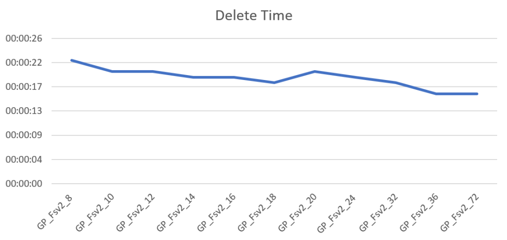
Delete data

After selecting data I decided I had enough of the large amount and had to trim some of. So I deleted 300.000 records. This process is quick all over the board, ranging from 22 seconds for the 8 core SKU to 16 seconds at best. With these differences it’s hard to make a case for more cores if deletes are your main goal.

The wait types:

The log writes take 41 percent of the waits again driving home the point that the fully logged recovery model has it’s drawbacks. The pwait takes 26 percent followed by the extended events with 18 percent. The PVS wait has 9 percent, the pagelatch 2 percent and finally locking takes a little over 1 percent. Now remember that the duration of the query’s is quite short, in a real life scenario things can turn out quite differently, though the waits most certainly will be there.

The read latency varied between 20 and 66 ms, averaging at 35 ms. The write latency varied between 21 and 118 ms averaging at 65 ms. The really weird outlier is at the 72 core SKU. It looks like not only the cores doubled but the write latency as well. Maybe the disks were unable to keep up with the cores, but the wait’s didn’t really show anything in that direction other than the regular log waits. Looking at these stats you’ve best of in the low SKU’s.

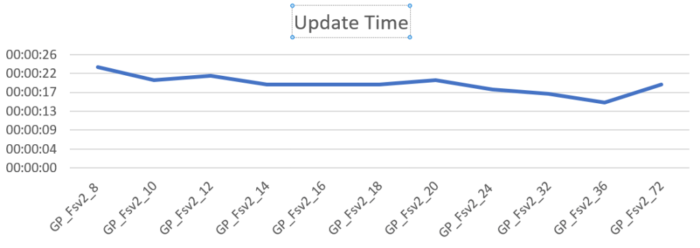
Update data

The last job I let rip on the database was an update task. I ran a script to update 300.000 records. The 8 core took 23 seconds, 72 core took 19. The behavior is quite the same as with deletes.

Let’s take a final look at the waits

Just two relevant ones. The one you’ll hit the most with 73 percent of the time is the page modification wait. Not really unexpected with a load of updates running. The extended events are just telling the portal what’s happening.

Let’s see if the disk latency is as weird as it was with the deletes.

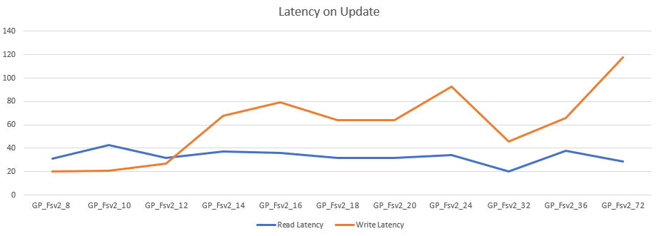
The latency is comparable with the update graph. Read between 29 and 43 ms, averaging at 33 ms. Write latency varied between 20 and 118 ms, averaging at 60 ms. And again at the 72 core a huge rise in latency. The rest seems a bit more cooperative though the same conclusion springs to mind; stay at the low end for the updates if you don’t want to get hit with a lot of extra disk latency.

Pricing

The pricing shows an even line over the different SKU’s. The breaks you’re seeing in the lines are caused by the uneven rises in cores. In the end, you’re paying a price per core (82,23 in my case) so there’s predictability again.

More performance will cost more and you’ll have to decide if this tier and it’s SKU is worth the cost. To keep this under control I’d advise you to use the cost center and it’s alerts. Not only the actual costs, you can create cost alerts on predicted costs as well to prevent surprises. We’ve all been there.

Finally

Now this is a very interesting SKU. It offers quite impressive compute performance in regard to price. 72 cores for less than 6000 per month sounds like nice value for money. The other tiers are somewhat more expensive in that regard. The general purpose tier costs 10 euro’s per month more. Then again, that tier offers more memory and TempDB. In this case, this tier will really work for you when you are really using the compute and less disk and memory. For large, weekly ETL loads, this tier might fall short but for short daily or hourly loads this might really prove very useful! It’s a tier that has made it to my shortlist of Azure tiers.

Thanks for reading and next week, Hyperscale.

One thought on “Azure SQL Database Performance comparison part 6 of 9: General Purpose Compute Optimized”

Pingback: Azure SQL DB GP Compute Optimized Performance Comp – Curated SQL

Azure SQL Database Performance comparison part 6 of 9: General Purpose Compute Optimized

Intro

Limits

Resources provided