Fooling around with TPC-H data, ADF and Hyperscale Serverless

In one of my last blogs, I wrote about my first encounter with the Azure Hyperscale Serverless offering. Now it’s time to dig a bit deeper and what it’s up to.

Disclaimer. Azure Hyperscale Serverless is in preview and one of the things that isn’t active yet, is the auto shutdown. This means that it will stay online 24/7. And bill you for every second it’s online. In my case, this meant that my Visual Studio credits ran out and I couldn’t use my Azure subscription anymore. Keep it in mind when testing this out, especially if your credit card is connected to said subscription.

Setup

To get the data, I downloaded and compiled the TPC-H data generator and created 500 GB of data files in 5 iterations. The process generates 5 sets of 8 files, each set being about 100 GB. This way, I hoped to get some parallelism reading the data. The LineItem file is the biggest one with not only the most records (over three billion) but also in size (a little over 400 GB).

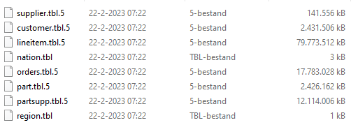
The storage account is a standard hot tier blob storage, no hierarchical namespace enabled. Uploading the files took about 10 hours, creating the files about 35 hours on a 10 year old Intel Core i5 machine.

The Hyperscale database was configured in the Serverless option with a maximum of 16 cores, minimum was automatically set at 2 cores. The tables were created with the correct schema, no indexes, (foreign) keys or other tricks were used. You can find the schema I’ve used here.

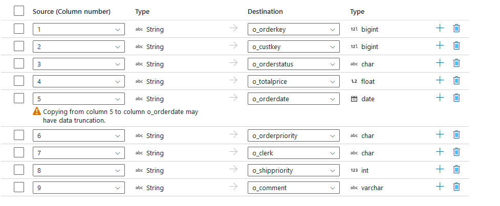
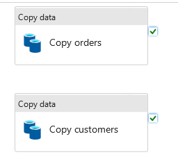
Finally, I used Azure Data Factory copy flows to get the data from the storage to the database. The schema was imported from the database and some conversion can take place when reading the data and writing it to the database.

Those who know the TPC-H output will find that I’m not writing on all the tables. I did load all of them, but took out the small, medium, large and extra large ones for readability. The smallest ones (region and nation) are discarded as their size doesn’t make sense in this test case.

Test 1: CSV to SQL

My first try was to get all the data from the CSV files into the SQL instance. I created the flows to read the the files and directly write into the database. As the tables have no indexes, I expected a lot from both data factory (that had no limits specified) and the database (that had to welcome all the data with open arms).

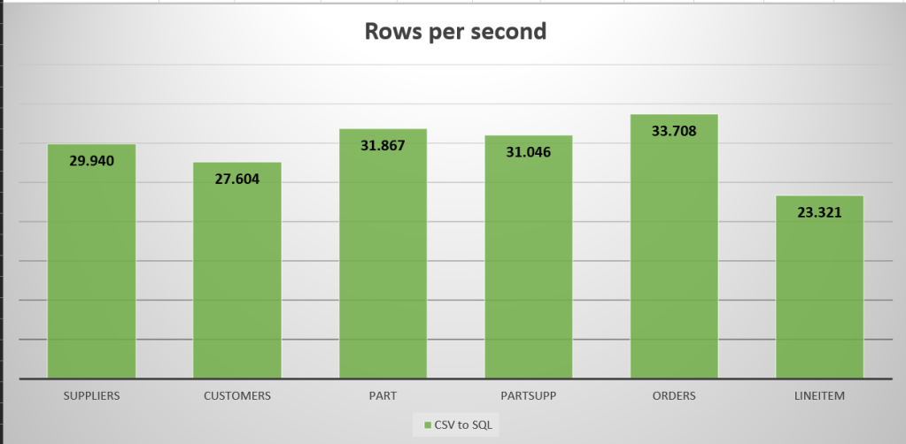
Let’s see what happened. The smallest table (Suppliers, 723 MB) took a little under three minutes to load. It grew to almost 1,5 GB in size and when the 5 million rows were loaded, the performance was about 29.940 records per second.

One of the medium sized tables (Part) with 100 million rows (12,5 GB) took 52 minutes to load and had an average speed of 31.867 rows per second. This one grew to 21 GB in SQL data.

The Orders table (90 GB, 750 million rows) took over 6 hours to load, grew to 136 GB and averaged at 33.708 rows per second.

The really big one, LineItem, timed out after 12 hours. I forgot to change the maximum run time. In that time, it managed to transfer a little over 1 billion rows to the SQL database, growing the data from 136 to 178 GB. It averaged a speed of 23.321 rows per second.

The different copy flows had 4 used DIUs and 2 used parallel copies. They had 20 peak connections at the source, 2 at the sink.

Let’s see the speed in a graph:

Now, the Azure storage reportedly works better with parquet files, so let’s try that!

CSV to Parquet

I created new copy data flows that read the CSV files and write them to parquet files. To give all the processes the ability to go as parallel as they wish, I’ve set the parquet sink to split the files in sets of 1 million rows. From a size point of view, maybe on the small side but file sizing is another discussion ;).

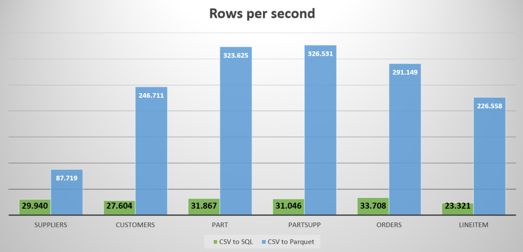
The smallest table (Suppliers, 723 MB) took a little under a minute to process. The volume shrunk to a little over 400 MB and when the 5 million rows were loaded, the performance averaged at 87.719 rows per second.

The medium sized table (Part) with 100 million rows (12,5 GB) took 5 minutes to load and had an average speed of 323.625 rows per second. This one shrunk to 4,5 GB in Parquet data.

The Orders table (90 GB, 750 million rows) took a little over 42 minutes to process, shrunk to 42 GB and averaged at 291.149 rows per second.

The really big one, LineItem didn’t time out. It finished in 3 hours and 40 minutes. Processing 3.000.028.242 rows shrinking it from 407 to 187 GB and averaging at 226.588 rows per second.

The different copy flows had 20 used DIUs and 5 used parallel copies. They had 50 peak connections at the source, 5 at the sink. A huge increase compared to the CSV to SQL load. The flows had the same settings as the CSV to SQL flows. This is just Azure Data Factory having a better time copying data from one folder to another one with a better(?) data type.

Let’s see this in a graph, compared to CSV to SQL:

Parquet to SQL

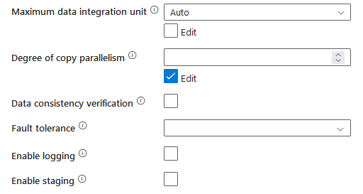
Now to get the data from parquet to sql. As I found that the standard settings for the data flows were insufficient, I changed some settings to increase performance. Changing the DIU and copy parallelism settings greatly increases performance, but it also increases cost. As I found out when my subscription locked again.

The smallest table (Suppliers, 823 MB read) took a little under four minutes to load. It grew to almost 1,5 GB in size and when the 5 million rows were loaded, the performance was about 22.422 records per second.

One of the medium sized tables (Part) with 100 million rows (9 GB read) took 41 minutes to load and had an average speed of 39.952 rows per second. This one grew to 21 GB in SQL data. The part copy flow has the same settings as Suppliers.

The Orders table (81 GB read, 750 million rows) took about 2,5 hours to load, grew to 136 GB and averaged at 86.846 rows per second.

The really big one, LineItem, finished as well. With 375 GB read, it transferred the 3 billion rows in a little under 7,5 hours. The data grew to 532 GB in the SQL DB but the process managed 111.704 rows per second.

For this last process, Suppliers and part were running with a max DIU of 8, Orders had 16 and LineItems 32. That is a lot of computing power. The copy parallelism was set to 8 across all tables. This meant that peak connections to the target went up to 8 for most tables, LineItem got 16 to write to the SQL DB. Let’s add the graphs to the previous one and see the differences.

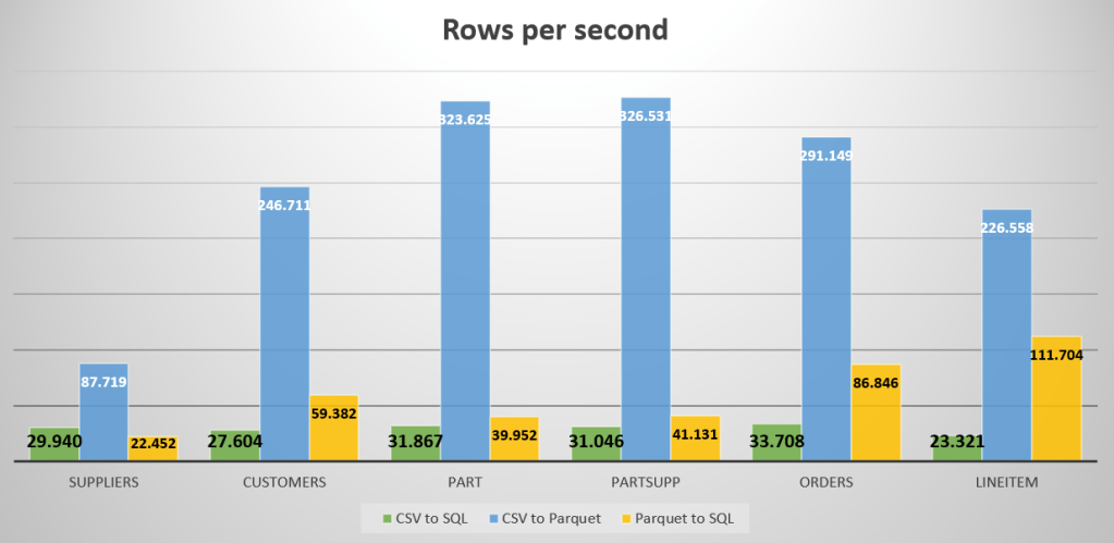
When you compare just the graphs, it seems that the best way forward is CSV to Parquet. Thing is, most people don’t speak parquet but speak SQL or Python. So you need to read the data again in either Synapse Studio, Synapse Serverless Database or even a dedicated SQL Pool to make the most out of the data.

Costs

As I started with, performance comes at a price.

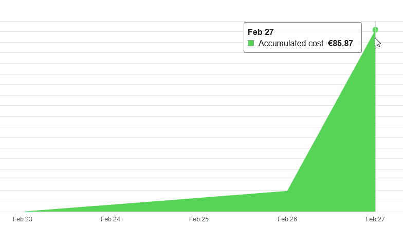
You can see quite clearly that between february 26th and 27th, I spent more money on my data factory. Increasing the DIU’s make huge difference.

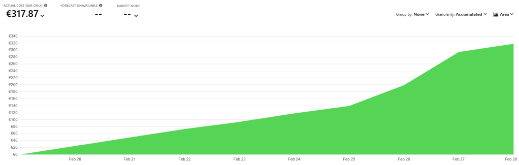
My database costs went through the roof as well, no wonder with a Hyperscale on 24/7.

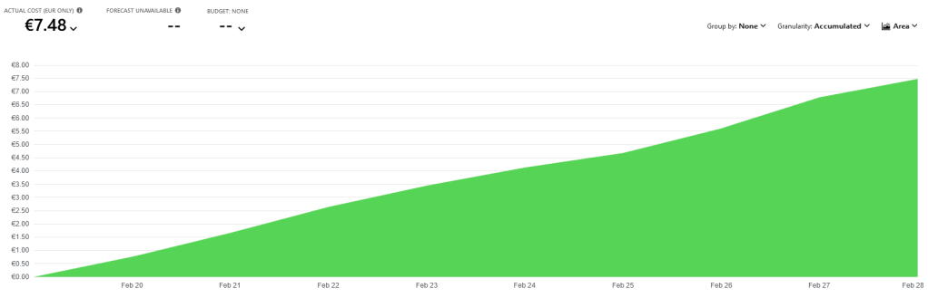
The costs of storing a little over 500 GB of data on storage is almost nothing compared to SQL data storage.

Resource usage

Now, how hard are my resources working? It’s ok that they cost money, but I’m expecting a lot in return. The data factory has shut down so hard, none of the graphs are returning any data, so let’s look at the Azure SQL database.

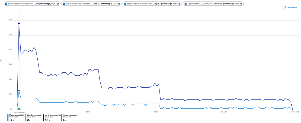
When the loading process starts, there’s a peak with 13% CPU (about 2 cores) and 58% Log IO. After the initial peak, the usage quickly drops down to almost a trickle. This concurs with the performance seen at the ADF side of things. It was calmly strolling along, reading and writing the data whilst taking in the spring smells and sun.

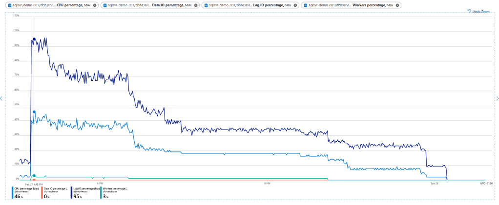
In general, the graph looks more or less the same. But the CPU reaches almost 50% at it’s peak moment, so almost 8 cores out the available 16 were used. The log IO almost hit the max but quickly decreased. What doesn’t cease to amaze me is the fact that the data IO remains at 0%. As the data is being processed by the distributed compute under the Hyperscale front, I can only imagine that the default monitoring query’s by Azure can’t read that part. Hopefully this will come in the near future as it’s a very welcome addition to the other data when analysing the tier and SKU settings.

Tables

To finish of this blog, I’ll leave you with three matrices of data collected during the running of the Data Factory processes. One of the things worth paying attention to is the amount of data read and data written. It’s noteworthy that when reading parquet, there’s more data read then there was written; the data needs to be decompressed and this generates overhead in the data read.

CSV to SQL

	Suppliers	Customers	Part	PartSupp	Orders	LineItem
Data Read	723 MB	12,438 GB	12,411 GB	61,979GB	90,77 GB	136,155 GB
Files Read	5	5	5	5	5	2
Rows Read	5.000.000	75.000.000	100.000.000	400.000.000	750.000.000	1.007.478.970
Peak Connections	50	20	20	20	20	20
Data Written	1,305 GB	22,425 GB	21,285 GB	111,6 GB	136.349 GB	178,885 GB
Rows Written	5.000.000	75.000.000	100.000.000	400.000.000	750.000.000	1.007.405.315
Peak Connections	8	2	2	2	2	2
Copy Duration	00:02:47	00:45:17	00:52:18	03:34:44	06:10:50	12:00:00
Throughput	4,468MB/s	4,588 MB/s	3,961 MB/s	4,812MB/s	4,081MB/s	3,152 Mb/s
Used DIUs	8	4	4	4	4	4
Used Parallel copies	8	2	2	2	2	2
Reading from source	00:00:09	00:18:11	00:16:06	01:57:26	02:11:24	04:15:00
Writing to sink	00:01:21	00:32:19	00:28:53	02:22:18	04:06:42	05:51:55
Rows per hour	107.784.431	99.374.310	114.722.753	111.766.532	121.348.315	83.956.581
Rows per minute	1.796.407	1.656.238	1.912.046	1.862.776	2.022.472	1.399.276
Rows per second	29.940	27.604	31.867	31.046	33.708	23.321

CSV to Parquet

	Suppliers	Customers	Part	PartSupp	Orders	LineItem
Data Read	723 MB	12,438 GB	12,411 GB	61,979GB	90,77 GB	407,322 GB
Files Read	5	5	5	5	5	5
Rows Read	5.000.000	75.000.000	100.000.000	400.000.000	750.000.000	3.000.028.242
Peak Connections	50	50	50	50	50	50
Data Written	411,659 MB	6,592 GB	4,528 GB	23,018 GB	42,034 GB	187,263 GB
Files written	5	75	100	400	750	3003
Rows Written	5.000.000	75.000.000	100.000.000	400.000.000	750.000.000	3.000.028.242
Peak Connections	5	5	5	5	5	5
Copy Duration	00:00:57	00:05:04	00:05:09	00:20:25	00:42:56	03:40:40
Throughput	13,919 MB/s	41.738 MB/s	40,825 MB/s	50,844 MB/s	35,319 MB/s	30,776 MB/s
Used DIUs	8	20	20	20	20	20
Used Parallel copies	5	5	5	5	5	5
Reading from source	00:00:06	00:01:55	00:01:33	00:11:23	00:20:46	01:35:24
Writing to sink	00:00:07	00:02:08	00:01:02	00:06:32	00:13:47	00:56:53
Rows per hour	315.789.474	888.157.895	1.165.048.544	1.175.510.204	1.048.136.646	815.717.649
Rows per minute	5.263.158	14.802.632	19.417.476	19.591.837	17.468.944	13.595.294
Rows per second	87.719	246.711	323.625	326.531	291.149	226.588

Parquet into SQL

	Suppliers	Customers	Part	PartSupp	Orders	LineItem
Data Read	823,328 MB	13,185 GB	9,056	46,037 GB	81,075	374,537 GB
Files Read	5	75	100	400	750	3003
Rows Read	5.000.000	75.000.000	100.000.000	400.000.000	750.000.000	3.000.028.242
Peak Connections	5	4	8	8	8	8
Data Written	1,305 GB	22,425 GB	21,285 GB	111,6 GB	136,349 GB	532,717 GB
Rows Written	5.000.000	75.000.000	100.000.000	400.000.000	750.000.000	3.000.028.242
Peak Connections	8	4	8	8	8	16
Copy Duration	00:03:43	00:21:03	00:41:43	02:42:05	02:23:56	07:27:37
Throughput	3,794 MB/s	10,481 MB/s	3,625 MB/s	4,737 MB/s	9,742 MB/s	13,948 MB/s
Used DIUs	4	8	8	8	16	32
Used Parallel copies	8	4	8	8	8	8
Reading from source	00:00:11	00:05:41	00:07:54	00:49:50	00:16:00	00:16:03
Writing to sink	00:02:15	00:18:56	00:21:30	01:11:41	02:07:44	07:23:18
Rows per hour	80.717.489	213.776.722	143.827.407	148.071.979	312.644.743	402.133.584
Rows per minute	1.345.291	3.562.945	2.397.123	2.467.866	5.210.746	6.702.226
Rows per second	22.422	59.382	39.952	41.131	86.846	111.704

Finally

Thank you so much for reading and many thanks to Henk van der Valk (T | B | L) for pointing me to the TCP-H data for more intens performance testing!